Ray Tracing in One Weekend:

Part Two - The First Weekend

19 Jun 2020

Now that we’re familiar with ray tracing through my introduction, we can delve into the titular first section of Peter Shirley’s book.

I started this path tracer months ago, and only started this blog in late May. The version of Shirley’s book that I used is from some time in 2018 (Version 1.54), and I have found that there is a recently updated version (3.1.2) on his website from June 6th, 2020! I also supplemented Shirley’s book with Victor Li’s posts on the subject. As such, there may be differences in implementation compared to the most recent version of Ray Tracing in One Weekend.

I am trying to keep things easy-to-follow, mostly sticking with my original code and only changing or adding what I deem to be necessary for readability, clarity, or image rendering purposes. If you are reading this to build your own ray tracer, I highly recommend Shirley’s book as a primary source.

---

Contents

• Image Output
• Timing Execution
• Vec3 Class
  • Vector Refresher
  • Vec3 Definitions
• Rays
  • Sending Rays from the Camera
• Introducing Spheres
  • Describing a Sphere
  • Placing a Sphere
• Surface Normals
  • Simplifying Ray-Sphere Intersection
• Multiple Spheres with the Hittable Class
• Front Faces Versus Back Faces
• Anti-Aliasing
  • Adding Anti-Aliasing to the Camera
• Diffuse Materials
  • The Math of Diffuse Materials
  • Gamma Correction
  • Shadow Acne
  • True Lambertian Reflection
• Common Constants and Utilities
• Metal
  • Abstract Class for Materials
  • Describing Ray-Object Intersections
  • Light Scatter
  • Metal Reflection
  • Adding Metal Spheres to the Scene
  • Fuzzy Metal
• Dielectrics
  • Refraction
  • Snell’s Law
  • Total Internal Reflection
  • Calculating the Refraction Vector
  • Coding the Refraction Vector
  • Dielectric Reflections
  • Hollow Dielectric Spheres
• Camera Modeling
• Depth of Field
• Final Scene

---

Image Output

Of course, the first step with producing a pretty path traced image is to produce an image. The method suggested by Peter is a simple plaintext .ppm file. The following is an example snippet and image from Wikipedia:

P3
3 2
255
# The part above is the header
# "P3" means this is an RGB color image in ASCII
# "3 2" is the width and height of the image in pixels
# "255" is the maximum value for each color
# The part below is image data: RGB triplets
255   0   0  # red
  0 255   0  # green
  0   0 255  # blue
255 255   0  # yellow
255 255 255  # white
  0   0   0  # black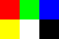

The code for creating a .ppm file is as follows:

main.cpp:

#include <iostream>

int main() {
	int nx = 200; // Number of horizontal pixels
	int ny = 100; // Number of vertical pixels
	std::cout << "P3\n" << nx << " " << ny << "\n255\n"; // P3 signifies ASCII, 255 signifies max color value
	for (int j = ny - 1; j >= 0; j--) { // Navigate canvas
	    std::cerr << "\rScanlines remaining: " << j << ' ' << std::flush;
		for (int i = 0; i < nx; i++) {
			float r = float(i) / float(nx);
			float g = float(j) / float(ny);
			float b = 0.2;
			int ir = int(255.99 * r);
			int ig = int(255.99 * g);
			int ib = int(255.99 * b);
			std::cout << ir << " " << ig << " " << ib << "\n";
		}
	}
	std::cerr << "\nDone.\n";
}

Note:

• Pixels are written from left to right.
• Rows of pixels are written top to bottom.
• In this simple example, from left to right, red goes from 0 to 255. Green goes from 0 to 255, bottom to top. As such, the top right corner should be yellow.

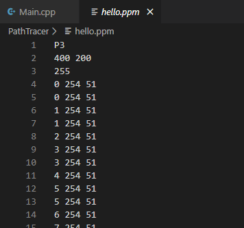
Now to compile and redirect the output of our program to a file:

g++ main.cpp
./a.out > hello.ppm

You may have to use a web tool or download a file viewer (I use IrfanView) to view the .ppm file as an image. Here’s my resulting image and raw contents of the file:

---

Timing Execution

Eventually, our program is going to chug when it comes to producing an image. It’s nice to have a total running time output. This is optional, and you can skip it if you please.

If you want, you could just run our program in the terminal prepended with time. Here’s an example of the utility:

eldun@Evan:/mnt/c/Users/Ev/source/Projects/PathTracer/PathTracer$ time sleep 1

real    0m1.019s
user    0m0.016s
sys     0m0.000s

Otherwise, you can #include <chrono> (for timing) and #include <iomanip> (for formatting) in main (or anywhere) to time more specific parts of the program:

#include <iostream>
#include <chrono>
#include <iomanip>


int main() {
	int nx = 200; // Number of horizontal pixels
	int ny = 100; // Number of vertical pixels
	std::cout << "P3\n" << nx << " " << ny << "\n255\n"; // P3 signifies ASCII, 255 signifies max color value

   		auto start = std::chrono::high_resolution_clock::now();	   

	for (int j = ny - 1; j >= 0; j--) { // Navigate canvas
	    std::cerr << "\rScanlines remaining: " << j << ' ' << std::flush;
		for (int i = 0; i < nx; i++) {
			float r = float(i) / float(nx);
			float g = float(j) / float(ny);
			float b = 0.2;
			int ir = int(255.99 * r);
			int ig = int(255.99 * g);
			int ib = int(255.99 * b);
			std::cout << ir << " " << ig << " " << ib << "\n";
		}
	}
		auto stop = std::chrono::high_resolution_clock::now(); 


	auto hours = std::chrono::duration_cast<std::chrono::hours>(stop - start);
	auto minutes = std::chrono::duration_cast<std::chrono::minutes>(stop - start) - hours;
	auto seconds = std::chrono::duration_cast<std::chrono::seconds>(stop - start) - hours - minutes;
    	std::cerr << std::fixed << std::setprecision(2) << "\nDone in:" << std::endl << 
	"\t" << hours.count() << " hours" << std::endl <<
	"\t" << minutes.count() << " minutes" << std::endl <<
	"\t" << seconds.count() << " seconds." << std::endl; 

}

---

Vec3 Class

Vectors! I feel like I haven’t used these since high school math but they are lovely. If you need or want a refresher on vectors, make sure to read this section. According to Peter Shirley, almost all graphics programs have some class(es) for storing geometric vectors and colors. In many cases, the vectors are four-dimensional to represent homogenous coordinates for geometry, or to represent the alpha transparency channel for color values. We’ll be using three-dimensional coordinates, as that’s all we need to represent direction, color, location, offset, etc.

Vector Refresher

Need a vector refresher? If so, check out this rundown at mathisfun.com. It’s the best I’ve found. All the operations within the code above are covered the mathisfun post. Take particular note of make_unit_vector(), dot(), and cross().

Here are the constructors and declarations of the functions we’ll be using within vec3.h.

vec3.h:

#ifndef VEC3H
#define VEC3H

#include <math.h>
#include <stdlib.h>
#include <iostream>

// 3 dimensional vectors will be used for colors, locations, directions, offsets, etc.
class vec3 {
public:
	vec3() {}
	vec3(double e0, double e1, double e2) { e[0] = e0; e[1] = e1; e[2] = e2; }

	inline double x() const { return e[0]; }
	inline double y() const { return e[1]; }
	inline double z() const { return e[2]; }
	inline double r() const { return e[0]; }
	inline double g() const { return e[1]; }
	inline double b() const { return e[2]; }

	// return reference to current vec3 object
	inline const vec3& operator+() const { return *this; }

	// return opposite of vector when using '-'
	inline vec3 operator-() const { return vec3(-e[0], -e[1], -e[2]); }

	// return value or reference to value of vec3 at index i ( I believe)
	inline double operator[](int i) const { return e[i]; }
	inline double& operator[](int i) { return e[i]; };

	inline vec3& operator+=(const vec3& v2);
	inline vec3& operator-=(const vec3& v2);
	inline vec3& operator*=(const vec3& v2);
	inline vec3& operator/=(const vec3& v2);
	inline vec3& operator*=(const double t);
	inline vec3& operator/=(const double t);

	inline double length() const {
		return sqrt(e[0]*e[0] + e[1]*e[1] + e[2]*e[2]);
	}
	inline double squared_length() const {
		return e[0]*e[0] + e[1]*e[1] + e[2]*e[2];
	}
	inline void make_unit_vector();

	double e[3];
};

...

Vec3 Definitions

The next step in our vector class is to define our functions. Be very careful here! This is where I had a few minor typo issues that mangled the final image later in the project. It’s not hard to see why; these are the lowest-level operations of vectors, which will simulate our light rays and their properties.

vec3.h:

...

// input output overloading
inline std::istream& operator>>(std::istream& is, vec3& t) {
	is >> t.e[0] >> t.e[1] >> t.e[2];
	return is;
}

inline std::ostream& operator<<(std::ostream& os, const vec3& t) {
	os << t.e[0] << " " << t.e[1] << " " << t.e[2];
	return os;
}


inline void vec3::make_unit_vector() {
	double k = 1.0 / sqrt(e[0]*e[0] + e[1]*e[1] + e[2]*e[2]);
	e[0] *= k;
	e[1] *= k;
	e[2] *= k;
}

inline vec3 operator+(const vec3& v1, const vec3& v2) {
	return vec3(v1.e[0] + v2.e[0], v1.e[1] + v2.e[1], v1.e[2] + v2.e[2]);
}

inline vec3 operator-(const vec3& v1, const vec3& v2) {
	return vec3(v1.e[0] - v2.e[0], v1.e[1] - v2.e[1], v1.e[2] - v2.e[2]);
}

inline vec3 operator*(const vec3& v1, const vec3& v2) {
	return vec3(v1.e[0] * v2.e[0], v1.e[1] * v2.e[1], v1.e[2] * v2.e[2]);
}

inline vec3 operator/(const vec3& v1, const vec3& v2) {
	return vec3(v1.e[0] / v2.e[0], v1.e[1] / v2.e[1], v1.e[2] / v2.e[2]);
}

inline vec3 operator*(double t, const vec3& v) {
	return vec3(t * v.e[0], t * v.e[1], t * v.e[2]);
}

inline vec3 operator/(const vec3 v, double t) {
	return vec3(v.e[0] / t, v.e[1] / t, v.e[2] / t);
}

inline vec3 operator*(const vec3& v, double t) {
	return vec3(t * v.e[0], t * v.e[1], t * v.e[2]);
}

// Dot product
inline double dot(const vec3& v1, const vec3& v2) {
	return
		v1.e[0] * v2.e[0]
		+ v1.e[1] * v2.e[1]
		+ v1.e[2] * v2.e[2];
}

// Cross product
inline vec3 cross(const vec3& v1, const vec3& v2) {
	return vec3(v1.e[1] * v2.e[2] - v1.e[2] * v2.e[1],
				v1.e[2] * v2.e[0] - v1.e[0] * v2.e[2],
				v1.e[0] * v2.e[1] - v1.e[1] * v2.e[0]);
}

inline vec3& vec3::operator+=(const vec3& v) {
	e[0] += v.e[0];
	e[1] += v.e[1];
	e[2] += v.e[2];
	return *this;
}
inline vec3& vec3::operator-=(const vec3& v) {
	e[0] -= v.e[0];
	e[1] -= v.e[1];
	e[2] -= v.e[2];
	return *this;
}

inline vec3& vec3::operator*=(const vec3& v) {
	e[0] *= v.e[0];
	e[1] *= v.e[1];
	e[2] *= v.e[2];
	return *this;
}

inline vec3& vec3::operator/=(const vec3& v) {
	e[0] /= v.e[0];
	e[1] /= v.e[1];
	e[2] /= v.e[2];
	return *this;
}

inline vec3& vec3::operator*=(const double t) {
	e[0] *= t;
	e[1] *= t;
	e[2] *= t;
	return *this;
}

inline vec3& vec3::operator/=(const double t) {
	double k = 1.0 / t;

	e[0] *= k;
	e[1] *= k;
	e[2] *= k;
	return *this;
}

inline vec3 unit_vector(vec3 v) {
	return v / v.length();
}

#endif // !VEC3H

Make sure to include our new vec3.h in main.cpp.

main.cpp:

#include <iostream>


#include "vec3.h"


int main() {
	int nx = 200; // Number of horizontal pixels
	int ny = 100; // Number of vertical pixels
	std::cout << "P3\n" << nx << " " << ny << "\n255\n"; // P3 signifies ASCII, 255 signifies max color value
	for (int j = ny - 1; j >= 0; j--) { // Navigate canvas
	    std::cerr << "\rScanlines remaining: " << j << ' ' << std::flush;
		for (int i = 0; i < nx; i++) {
			
			vec3 col(float(i) / float(nx), float(j) / float(ny), 0.2);
			int ir = int(255.99 * col[0]);
			int ig = int(255.99 * col[1]);
			int ib = int(255.99 * col[2]);
			
			std::cout << ir << " " << ig << " " << ib << "\n";
		}
	}
    std::cerr << "\nDone.\n";
}

---

Rays

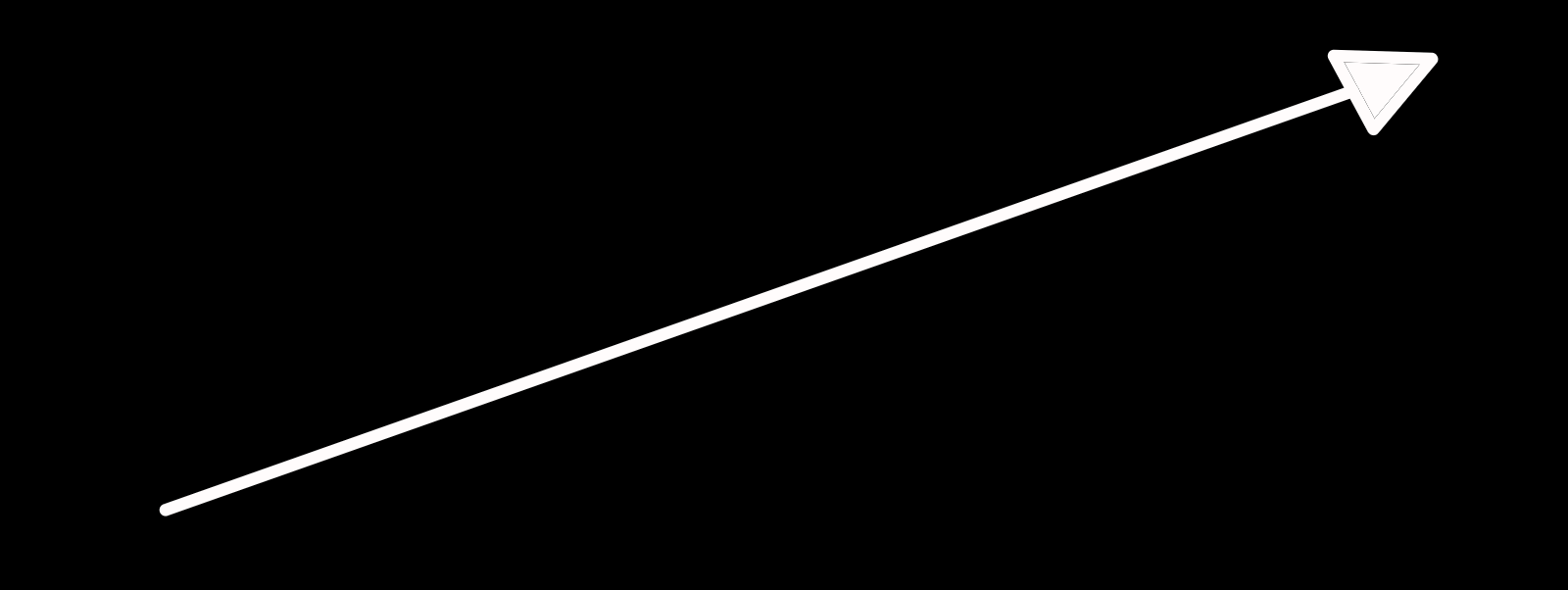
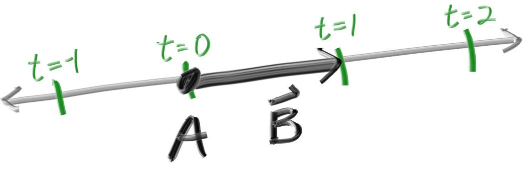
Ray tracers need rays! These are what will be colliding with objects in the scene. Rays have an origin, a direction, and can be described by the following formula:

P(t) = A + tB

• p is a point on the ray.
• A is the ray origin.
• B is the direction of the ray.
• The ray parameter t is a real number (positive or negative) that moves p(t) along the ray.

Here’s the header file for our ray class:

ray.h:

#ifndef RAYH
#define RAYH
#include "Vec3.h"

class ray
{
public:
	ray() {}
	ray(const vec3& a, const vec3& b) { A = a; B = b; }
	vec3 origin() const		{ return A; }
	vec3 direction() const	{ return B; }
	vec3 point_at_parameter(double t) const { return A + t * B; }

	vec3 A;
	vec3 B;
};

#endif // !RAYH

Sending Rays from the Camera

Put simply, our ray tracer will send rays through pixels and compute the color seen for each ray. The steps for doing so are as follows:

1. Calculate the ray from camera to pixel.
2. Determine which objects the ray intersects.
3. Compute a color for the intersection.

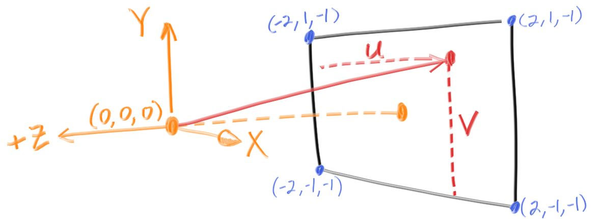
We will need a “viewport” of sorts to pass rays through from our “camera.” Since we’re using standard square pixel spacing, the viewport will have the same aspect ratio as our rendered image. Shirley sets the height of the viewport to two units in his book, and we’ll do the same.

Using Peter Shirley’s example, we’re going to set the camera at (0,0,0), and look towards the negative z-axis. The viewport will be traversed with rays from left-to-right, bottom-to-top. Variables u and v will be the offset vectors used to move the camera ray along the viewport:

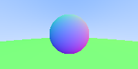
Here’s our code for the camera, as well as rendering a blue-to-white gradient:

main.cpp:

#include <iostream>
#include "ray.h"

/*
* Linearly blends white and blue depending on the value of y coordinate (Linear Blend/Linear Interpolation/lerp).
* Lerps are always of the form: blended_value = (1-t)*start_value + t*end_value.
* t = 0.0 = White
* t = 1.0 = Blue
*/
vec3 color(const ray& r) {
	vec3 unit_direction = unit_vector(r.direction());
	double t = 0.5 * (unit_direction.y() + 1.0);
	return (1.0 - t) * vec3(1.0, 1.0, 1.0) + t * vec3(0.5, 0.7, 1.0);

}

int main() {
	int nx = 200; // Number of horizontal pixels
	int ny = 100; // Number of vertical pixels
	std::cout << "P3\n" << nx << " " << ny << "\n255\n"; // P3 signifies ASCII, 255 signifies max color value

	// The values below are derived from making the "camera"/ray origin coordinates (0, 0, 0) relative to the canvas.
	vec3 lower_left_corner(-2.0, -1.0, -1.0);
	vec3 horizontal(4.0, 0.0, 0.0);
	vec3 vertical(0.0, 2.0, 0.0);
	vec3 origin(0.0, 0.0, 0.0);
	for (int j = ny - 1; j >= 0; j--) {
		std::cerr << "\rScanlines remaining: " << j << ' ' << std::flush;
		for (int i = 0; i < nx; i++) {
			double u = double(i) / double(nx);
			double v = double(j) / double(ny);

			// Approximate pixel centers on the canvas for each ray r
			ray r(origin, lower_left_corner + u * horizontal + v * vertical);

			vec3 col = color(r);
			int ir = int(255.99 * col[0]);
			int ig = int(255.99 * col[1]);
			int ib = int(255.99 * col[2]);
			std::cout << ir << " " << ig << " " << ib << "\n";
		}
	}
	std::cerr << "\nDone.\n";
}

The result:

We can move the camera code into camera.h.

camera.h:

#ifndef CAMERAH
#define CAMERAH

#include "ray.h"

class camera {
public:

	// The values below are derived from making the "camera" / ray origin coordinates(0, 0, 0) relative to the canvas.
	camera() {
		lower_left_corner = vec3(-2.0, -1.0, -1.0);
		horizontal = vec3(4.0, 0.0, 0.0);
		vertical = vec3(0.0, 2.0, 0.0);
		origin = vec3(0.0, 0.0, 0.0);
	}
	ray get_ray(double u, double v) { return ray(origin, lower_left_corner + u * horizontal + v * vertical - origin); }

	vec3 origin;
	vec3 lower_left_corner;
	vec3 horizontal;
	vec3 vertical;
};

#endif // !CAMERAH

---

Introducing Spheres

Describing a Sphere

We have a beautiful sky-like gradient. Let’s add a sphere! Spheres are popular in ray tracers because they’re mathematically simple.

A sphere centered at the origin of radius $R$ is $x^2 + y^2 + z^2 = R^2$.

• This means that if a point $(x,y,z)$ is on a sphere, $x^2 + y^2 + z^2 = R^2$.
• If the point is inside the sphere, $x^2 + y^2 + z^2 < R^2$.
• If the point is outside the sphere, $x^2 + y^2 + z^2 > R^2$

If the sphere center isn’t at the origin, the formula is:

\[(x - C_x)^2 + (y - C_y)^2 + (z - C_z)^2 = r^2\]

It’s best if formulas are kept under the hood in the vec3 class.

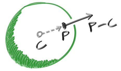
The vector from center $\mathbf{C} = (C_x,C_y,C_z)$ to point $\mathbf{P} = (x,y,z)$ is $(\mathbf{P} - \mathbf{C})$, and therefore

\[(\mathbf{P} - \mathbf{C}) \cdot (\mathbf{P} - \mathbf{C}) = (x - C_x)^2 + (y - C_y)^2 + (z - C_z)^2\]

Therefore, the equation of a sphere in vector form is:

\[(\mathbf{P} - \mathbf{C}) \cdot (\mathbf{P} - \mathbf{C}) = r^2\]

Any point $\mathbf{P}$ that satisfies this equation is on the sphere. We’re going to find out if a given ray ever hits the sphere. If it does, there is a value t for which P(t) satisfies this equation:

\[(\mathbf{P}(t) - \mathbf{C}) \cdot (\mathbf{P}(t) - \mathbf{C}) = r^2\]

The same formula, expanded:

\[(\mathbf{A} + t \mathbf{b} - \mathbf{C}) \cdot (\mathbf{A} + t \mathbf{b} - \mathbf{C}) = r^2\]

and again:

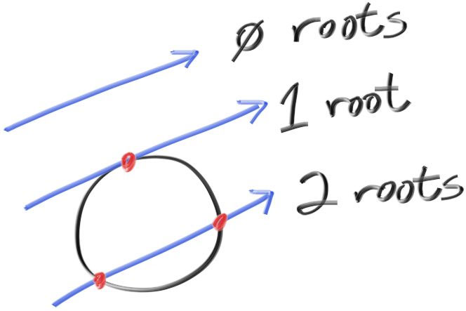
\[t^2 \mathbf{b} \cdot \mathbf{b} + 2t \mathbf{b} \cdot (\mathbf{A}-\mathbf{C}) + (\mathbf{A}-\mathbf{C}) \cdot (\mathbf{A}-\mathbf{C}) - r^2 = 0\]

The unknown variable is t, and this is a quadratic equation. Solving for t will lead to a square root operation (aka the discriminant) that is either positive (two real solutions), negative (no real solutions), or zero (one real solution):

Placing a Sphere

Prepend main.cpp’s main function with the following to mathematically hard-code a sphere to be hit by rays:

main.cpp:

...

bool hit_sphere(const vec3& center, double radius, const ray& r) {
	vec3 oc = r.origin() - center;
	double a = dot(r.direction(), r.direction());
	double b = 2.0 * dot(oc, r.direction());
	double c = dot(oc, oc) - radius * radius;
	double discriminant = b*b - 4*a*c;
	return (discriminant > 0);
}

/*
* Linearly blends white and blue depending on the value of y coordinate (Linear Blend/Linear Interpolation/lerp).
* Lerps are always of the form: blended_value = (1-t)*start_value + t*end_value.
* t = 0.0 = White
* t = 1.0 = Blue
*/
vec3 color(const ray& r) {
	if (hit_sphere(vec3(0, 0, -1), 0.5, r))
		return vec3(1, 0, 0);
	vec3 unit_direction = unit_vector(r.direction());
	double t = 0.5 * (unit_direction.y() + 1.0);
	return (1.0 - t) * vec3(1.0, 1.0, 1.0) + t * vec3(0.5, 0.7, 1.0);
}

...

The result:

---

Surface Normals

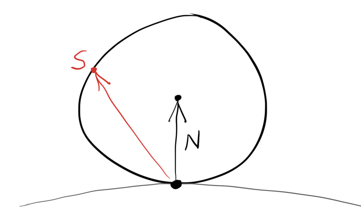
Our sphere looks like a circle. To make it more obvious that it is a sphere, we’ll add surface normals to the face. Surface normals are simply vectors that are perpendicular to the surface of an object.

In our case, the outward normal is the hitpoint minus the center:

Since we don’t have any lights, we can visualize the normals with a color map.

Our main.cpp file will now look something like this:

main.cpp:

#include <iostream>
#include "ray.h"

double hit_sphere(const vec3& center, double radius, const ray& r) {
	vec3 oc = r.origin() - center;
	double a = dot(r.direction(), r.direction());
	double b = 2.0 * dot(oc, r.direction());
	double c = dot(oc, oc) - radius * radius;
	double discriminant = (b*b) - (4*a*c);
	if (discriminant < 0) {
		return -1.0;
	}


	else {
		return (-b - sqrt(discriminant)) / (2.0 * a);
}
}

/*
* Assign colors to pixels
*
* Background -
* Linearly blends white and blue depending on the value of y coordinate (Linear Blend/Linear Interpolation/lerp).
* Lerps are always of the form: blended_value = (1-t)*start_value + t*end_value.
* t = 0.0 = White
* t = 1.0 = Blue
* 
* Draw sphere and surface normals
*/
vec3 color(const ray& r) {
	double t = hit_sphere(vec3(0, 0, -1), 0.5, r); // does the ray hit the values of a sphere placed at (0,0,-1) with a radius of .5?
	if (t > 0.0) { // sphere hit
		vec3 N = unit_vector(r.point_at_parameter(t) - vec3(0, 0, -1)); // N (the normal) is calculated
		return 0.5 * (vec3(N.x() + 1, N.y() + 1, N.z() + 1)); // RGB values assigned based on xyz values
	}
	vec3 unit_direction = unit_vector(r.direction());
	t = 0.5 * (unit_direction.y() + 1.0);
	return (1.0 - t) * vec3(1.0, 1.0, 1.0) + t * vec3(0.5, 0.7, 1.0);

}

...

Our resulting image:

Simplifying Ray-Sphere Intersection

As it turns out, we can simplify ray-sphere intersection. Here’s our original equation:

vec3 oc = r.origin() - center;
auto a = dot(r.direction(), r.direction());
auto b = 2.0 * dot(oc, r.direction());
auto c = dot(oc, oc) - radius*radius;
auto discriminant = b*b - 4*a*c;

The dot product of a vector with itself is equal to the squared length of that vector.

Additionally, the equation for b has a factor of two in it. Consider the quadratic equation if b = 2h:

\[\frac{-b \pm \sqrt{b^2 - 4ac}}{2a}\] \[= \frac{-2h \pm \sqrt{(2h)^2 - 4ac}}{2a}\] \[= \frac{-2h \pm 2\sqrt{h^2 - ac}}{2a}\] \[= \frac{-h \pm \sqrt{h^2 - ac}}{a}\]

As such, we can refactor our code like so:

vec3 oc = r.origin() - center;
auto a = r.direction().length_squared();
auto half_b = dot(oc, r.direction());
auto c = oc.length_squared() - radius*radius;
auto discriminant = half_b*half_b - a*c;

if (discriminant < 0) {
    return -1.0;
} else {
    return (-half_b - sqrt(discriminant) ) / a;
}

Cool! But it could be cooler. We need more spheres. The cleanest way to accomplish this is to create an abstract class - a class that must be overwritten by derived classes - of hittable objects.

---

Multiple Spheres with the Hittable Class

Our hittable abstract class will have a “hit” function that will be passed a ray and a record containing information about the hit, such as the time(which will be added with motion blur later in this series), position, and the surface normal:

hittable.h:

#ifndef HITTABLEH
#define HITTABLEH

#include "ray.h"


struct hit_record {
	double t;
	vec3 p;
	vec3 normal;
};

/* 
* A class for objects rays can hit.
*/
class hittable {
public:
	virtual bool hit(const ray& r, double t_min, double t_max, hit_record& rec) const = 0;
};

#endif // !HITTABLEH

---

Front Faces Versus Back Faces

A question we have to ask ourselves about our normals is whether they should always point outward. Right now, the normal will always be in the direction of the center to the intersection point - outward. So if the ray intersects from the outside, the normal is against the ray. If the ray intersects from the inside (like in a glass ball), the normal would be pointing in the same direction of the ray. The alternative option is to have the normal always point against the ray.

If we decide to always have the normal point outward, we need to determine what side the ray is on when we color it. If they face the same direction, the ray is inside the object traveling outward. If they’re opposite, the ray is outside traveling inward. We can determine this by taking the dot product of the ray and the normal - if the dot is positive, the ray is inside traveling outward.

if (dot(ray_direction, outward_normal) > 0.0) {
    // ray is inside the sphere
    ...
} else {
    // ray is outside the sphere
    ...
}

Suppose we take the other option: always having the normals point against the ray. We would have to store what side of the surface the ray is on:

bool front_face;
if (dot(ray_direction, outward_normal) > 0.0) {
    // ray is inside the sphere
    normal = -outward_normal;
    front_face = false;
}
else {
    // ray is outside the sphere
    normal = outward_normal;
    front_face = true;
}

You can choose whichever method you please, but Shirley’s book recommends the “outward” boolean method, as we will have more material types than geometric types for the time being.

Following the suggestion of Shirley, we’ll add a front_face boolean to the hittable.h hit_record struct, as well as a function to solve the calculation:

hittable.h:

#ifndef HITTABLEH
#define HITTABLEH

#include "ray.h"


struct hit_record {
	double t; // parameter of the ray that locates the intersection point
	vec3 p; // intersection point
	vec3 normal;
	bool front_face;
	
	inline void set_face_normal(const ray& r, const vec3& outward_normal) {
    		front_face = dot(r.direction(), outward_normal) < 0;
    		normal = front_face ? outward_normal :-outward_normal;
	} 
};

class hittable {
public: 
	virtual bool hit(const ray& r, double t_min, double t_max, hit_record& rec) const = 0;
};

#endif // !HITTABLEH

And now to update our sphere header with the simplified ray intersection and the outward normal calculations):

sphere.h:

#ifndef SPHEREH
#define SPHEREH

#include "hittable.h"

class sphere : public hittable {
public:
	sphere() {}
	sphere(vec3 cen, float r) : center(cen), radius(r) {};
	virtual bool hit(const ray& r, double tmin, double tmax, hit_record& rec) const;
	vec3 center;
	double radius;
};

bool sphere::hit(const ray& r, double t_min, double t_max, hit_record& rec) const {
	vec3 oc = r.origin() - center; // Vector from center to ray origin
	double a = r.direction().length_squared();
	double halfB = dot(oc, r.direction());
	double c = oc.length_squared() - radius*radius;
	double discriminant = (halfB * halfB) - (a * c);
	if (discriminant > 0.0) {
        auto root = sqrt(discriminant);

		auto temp = (-halfB - root)/a;

		if (temp < t_max && temp > t_min) {
			rec.t = temp;
			rec.p = r.point_at_parameter(rec.t);
vec3 outward_normal = (rec.p - center) / radius;
            rec.set_face_normal(r, outward_normal);
			return true;
		}
		temp = (-halfB + root / a;
		if (temp < t_max && temp > t_min) {
			rec.t = temp;
			rec.p = r.point_at_parameter(rec.t);
vec3 outward_normal = (rec.p - center) / radius;
            rec.set_face_normal(r, outward_normal);
			return true;
		}
	}
	return false;
}

#endif // !SPHEREH

As well as a new file for a list of hittable objects:

hittableList.h:

#ifndef HITTABLELISTH
#define HITTABLELISTH

#include "hittable.h"

class hittable_list : public hittable {
public:
	hittable_list() {}
	hittable_list(hittable** l, int n) { list = l; list_size = n; }
	virtual bool hit(const ray& r, double tmin, double tmax, hit_record& rec) const;
	hittable** list;
	int list_size;
};

bool hittable_list::hit(const ray& r, double t_min, double t_max, hit_record& rec) const {
	hit_record temp_rec;
	bool hit_anything = false;
	double closest_so_far = t_max;
	for (int i = 0; i < list_size; i++) {
		if (list[i]->hit(r, t_min, closest_so_far, temp_rec)) {
			hit_anything = true;
			closest_so_far = temp_rec.t;
			rec = temp_rec;
		}
	}
	return hit_anything;
}

#endif // !HITTABLELISTH

And the modified main.cpp:

main.cpp:

#include <iostream>
#include "sphere.h"
#include "hittableList.h"
#include "float.h"


/*
* Assign colors to pixels
*
* Background -
* Linearly blends white and blue depending on the value of y coordinate (Linear Blend/Linear Interpolation/lerp).
* Lerps are always of the form: blended_value = (1-t)*start_value + t*end_value.
* t = 0.0 = White
* t = 1.0 = Blue
* 
* Draw sphere and surface normals
*/
vec3 color(const ray& r, hittable * world) {
	hit_record rec;
	if (world->hit(r, 0.0, DBL_MAX, rec)) {
		return 0.5 * vec3(rec.normal.x() + 1, rec.normal.y() + 1, rec.normal.z() + 1); // return a vector with values between 0 and 1 (based on xyz) to be converted to rgb values
	}
	else { // background
		vec3 unit_direction = unit_vector(r.direction());
		double t = 0.5 * (unit_direction.y() + 1.0);
		return (1.0 - t) * vec3(1.0, 1.0, 1.0) + t * vec3(0.5, 0.7, 1.0);
	}
}

int main() {
	int nx = 200; // Number of horizontal pixels
	int ny = 100; // Number of vertical pixels
	std::cout << "P3\n" << nx << " " << ny << "\n255\n"; // P3 signifies ASCII, 255 signifies max color value

	// The values below are derived from making the "camera"/ray origin coordinates (0, 0, 0) relative to the canvas. 
	// See the included file "TracingIllustration.png" for a visual representation.
	vec3 lower_left_corner(-2.0, -1.0, -1.0);
	vec3 horizontal(4.0, 0.0, 0.0);
	vec3 vertical(0.0, 2.0, 0.0);
	vec3 origin(0.0, 0.0, 0.0);

	// Create spheres
	hittable *list[2];
	list[0] = new sphere(vec3(0, 0, -1), 0.5);
	list[1] = new sphere(vec3(0, -100.5, -1), 100);
	hittable* world = new hittable_list(list, 2);

	for (int j = ny - 1; j >= 0; j--) { // Navigate canvas
	    std::cerr << "\rScanlines remaining: " << j << ' ' << std::flush;
		for (int i = 0; i < nx; i++) {
			double u = double(i) / double(nx);
			double v = double(j) / double(ny);

			// Approximate pixel centers on the canvas for each ray r
			ray r(origin, lower_left_corner + u * horizontal + v * vertical);

			vec3 p = r.point_at_parameter(2.0);
			vec3 col = color(r, world);
			int ir = int(255.99 * col[0]);
			int ig = int(255.99 * col[1]);
			int ib = int(255.99 * col[2]);
			std::cout << ir << " " << ig << " " << ib << "\n";
		}
	}
	std::cerr << "\nDone.\n";
}

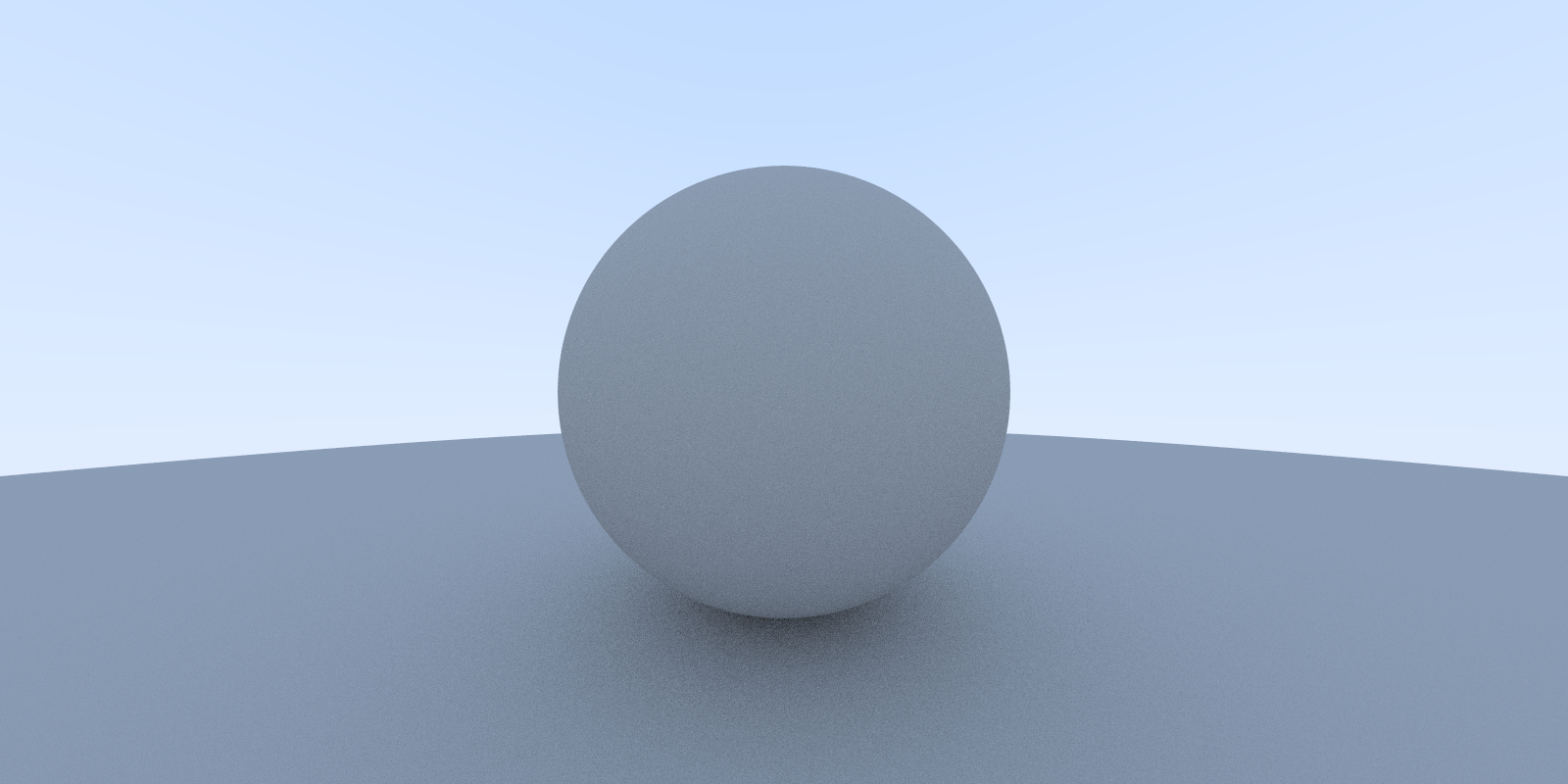
The result:

Stunning. A little bit jaggedy, though, don’t you think? This effect is known as “aliasing.” If you wanted to, you could increase the resolution of our scene for higher fidelity. Another interesting method for better image quality falls under the umbrella term “anti-aliasing.”

---

Anti-Aliasing

Anti-aliasing encompasses a whole slew of methods to combat “jaggies” - from multi-sampling to super-sampling, approximation(FXAA) to temporal, or - more recently - deep learning anti-aliasing. Each of these methods has pros and cons depending on the type of scene portrayed, performance targets, and even scene movement. Usually, there’s a trade-off between image quality and speed. We’ve entered a fascinating time for graphics where raw pixel count (True 4K this! Real 4K that!) is becoming less important - thanks to some incredible leaps in upscaling and anti-aliasing.

If you want to learn more, I highly suggest watching this video from one of my favorite YouTube channels(Digital Foundry), or reading this blog post from techguided.com.

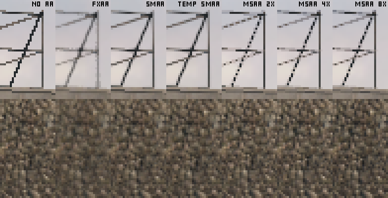
We’re going to be using multisample anti-aliasing (MSAA) in our ray tracer. As you may have supposed, multisampling, in this case, means taking multiple sub-pixel samples from each pixel and averaging the color across the whole pixel. Here’s an example - the raw triangle on the left, and the triangle with four samples per pixel on the right:

  [Source](https://developer.apple.com/documentation/metal/gpu_features/understanding_gpu_family_4/about_enhanced_msaa_and_imageblock_sample_coverage_control)

Instead of taking perfectly spaced samples of pixels like in the example above, we’ll be taking random samples of pixels. For that, we’ll need a way of generating random numbers (you can do it however you please):

random.h:

#ifndef RANDOMH
#define RANDOMH

#include <cstdlib>

inline double random_double() {
    // Returns a random real in [0,1).
    return rand() / (RAND_MAX + 1.0);
}

inline double random_double(double min, double max) {
    // Returns a random real in [min,max).
    return min + (max-min)*random_double();
}

#endif // !RANDOMH

Adding Anti-Aliasing to the Camera

Next, we’ll create a camera class to manage the virtual camera and scene sampling:

#ifndef CAMERAH
#define CAMERAH

#include "ray.h"

class camera {
public:

	// The values below are derived from making the "camera" / ray origin coordinates(0, 0, 0) relative to the canvas.
	camera() {
		lower_left_corner = vec3(-2.0, -1.0, -1.0);
		horizontal = vec3(4.0, 0.0, 0.0);
		vertical = vec3(0.0, 2.0, 0.0);
		origin = vec3(0.0, 0.0, 0.0);
	}
	ray get_ray(double u, double v) { return ray(origin, lower_left_corner + u * horizontal + v * vertical - origin); }

	vec3 origin;
	vec3 lower_left_corner;
	vec3 horizontal;
	vec3 vertical;
};

#endif // !CAMERAH

And our resulting main method:

main.cpp:

#include <iostream>
#include "sphere.h"
#include "hittableList.h"
#include "camera.h"
#include "random.h"


/*
* Assign colors to pixels
*
* Background -
* Linearly blends white and blue depending on the value of y coordinate (Linear Blend/Linear Interpolation/lerp).
* Lerps are always of the form: blended_value = (1-t)*start_value + t*end_value.
* t = 0.0 = White
* t = 1.0 = Blue
* 
*/
vec3 color(const ray& r, hittable * world) {
	hit_record rec;
	if (world->hit(r, 0.0, DBL, rec)) {
		return 0.5 * vec3(rec.normal.x() + 1, rec.normal.y() + 1, rec.normal.z() + 1); // return a vector with values between 0 and 1 (based on xyz) to be converted to rgb values
	}
	else { // background
		vec3 unit_direction = unit_vector(r.direction());
		double t = 0.5 * (unit_direction.y() + 1.0);
		return (1.0 - t) * vec3(1.0, 1.0, 1.0) + t * vec3(0.5, 0.7, 1.0);
	}
}

int main() {

	int nx = 200; // Number of horizontal pixels
	int ny = 100; // Number of vertical pixels
	int ns = 100; // Number of samples for each pixel for anti-aliasing
	std::cout << "P3\n" << nx << " " << ny << "\n255\n"; // P3 signifies ASCII, 255 signifies max color value

	// Create spheres
	hittable *list[2];
	list[0] = new sphere(vec3(0, 0, -1), 0.5);
	list[1] = new sphere(vec3(0, -100.5, -1), 100);
	hittable* world = new hittable_list(list, 2);
	camera cam;

	for (int j = ny - 1; j >= 0; j--) { // Navigate canvas
	    std::cerr << "\rScanlines remaining: " << j << ' ' << std::flush;
		for (int i = 0; i < nx; i++) {
			vec3 col(0, 0, 0);
			for (int s = 0; s < ns; s++) { // Anti-aliasing - get ns samples for each pixel
				double u = (i + random_double(0.0, 1)) / double(nx);
				double v = (j + random_double(0.0, 1)) / double(ny);
				ray r = cam.get_ray(u, v);
				vec3 p = r.point_at_parameter(2.0);
				col += color(r, world);
			}

			col /= double(ns); // Average the color between objects/background
			int ir = int(255.99 * col[0]);
			int ig = int(255.99 * col[1]);
			int ib = int(255.99 * col[2]);
			std::cout << ir << " " << ig << " " << ib << "\n";
		}
	}
    std::cerr << "\nDone.\n";
}

Keep in mind - these images are only 200x100. The difference is clear. And blurry. Haha:

---

Diffuse Materials

Our ball is pretty, but lacks texture. Let’s add diffuse materials!

Diffuse materials reflect light from their surface such that an incident ray is scattered ay many angles, rather than just one (which is the case with specular reflection):

An example of light reflecting off of a diffuse surface (source)

From Wikipedia:

The visibility of objects, excluding light-emitting ones, is primarily caused by diffuse reflection of light: it is diffusely-scattered light that forms the image of the object in the observer’s eye.

Diffuse materials also modulate the color of their surroundings with their intrinsic color. In our ray tracer, we’re going to simulate diffuse materials by randomizing ray reflections upon hitting a diffuse object. For example, if we were to shoot three rays into the space between two diffuse surfaces, we might see a result like this:

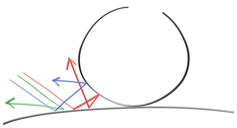How rays might behave in our ray tracer upon hitting a diffuse surface (source)

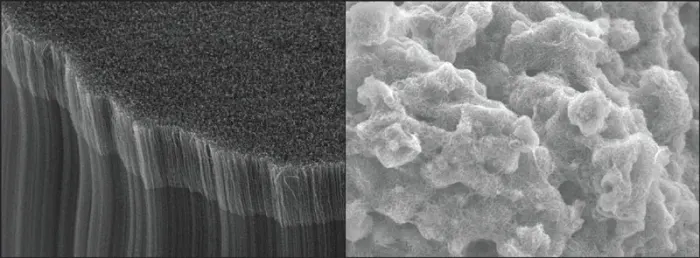
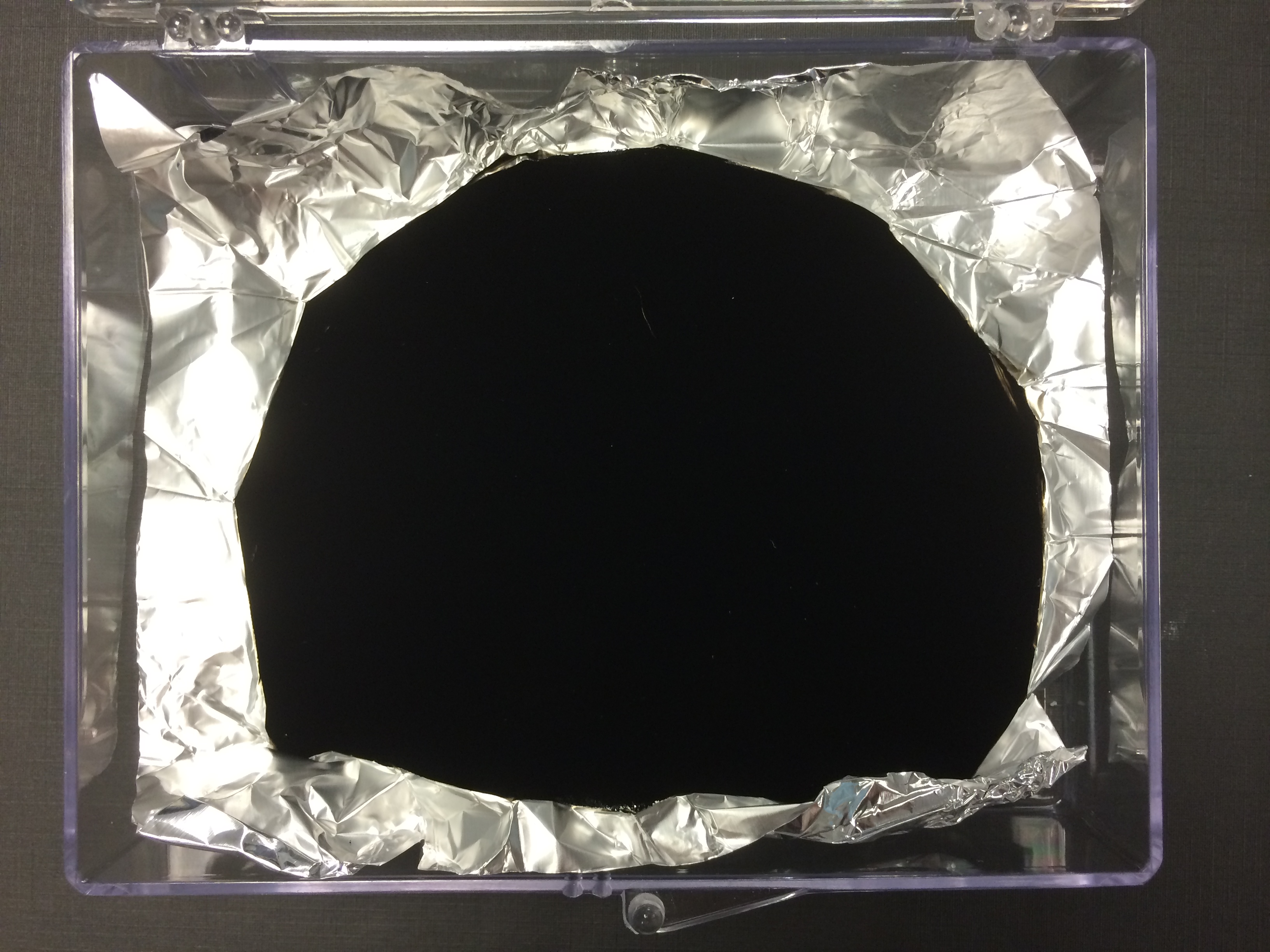
In addition to being reflected, some rays could also be absorbed. Naturally, the darker the surface of a given object, the more likely absorption will take place… which is why that object looks dark. Take Vantablack, one of the darkest substances known. It’s made up of carbon nanotubes, and is essentially a very fine shag carpet. Light gets lost (or diffused) within this forest of tubes to create a pretty striking diffuse material:

When I was originally reading Peter Shirley’s guide, he described an incorrect (but close) approximation of ideal Lambertian reflectance(think unfinished wood or charcoal - no shiny specular highlights). We’ll go through how I originally did it, and then modify the code to make matte surfaces more true-to-life, thanks to an update to his book.

The Math of Diffuse Materials

First of all, we need to form a unit sphere tangent to the hitpoint p on the scene object. The center of this sphere will be the coordinates at the end of the surface normal n. Be aware that there are two spheres tangential to the collided sphere - one inside the object(p - n), and one outside(p + n). we’ll pick the tangent sphere that’s on the same side of the surface as the ray origin. Next, we’ll select a random point s in the tangent unit sphere and send a ray from the hit point p to the random point s - which results in the vector s - p.

Generation of random diffuse bounce ray (source)

Now we need a way to pick the aforementioned random point s. Following Shirley’s lead, we’ll use a rejection method; picking a random point in the unit cube where x, y, and z all range from -1 to 1. If the point is outside the sphere (x² + y² + z² > 1), we reject it and try again:

vec3.h:

vec3 random_unit_sphere_coordinate() {
	vec3 p;
	do {
		p = 2.0 * vec3(random_double(0, 1), random_double(0, 1), random_double(0, 1)) - vec3(1, 1, 1);
	} while (p.squared_length() >= 1.0);
	return p;
}

Now we have to update our color function to use the random coordinates:

main.cpp:

vec3 color(const ray& r, hittable * world) {
	hit_record rec;
	// Light that reflects off a diffuse surface has its direction randomized.
	// Light may also be absorbed.
	if (world->hit(r, 0.0, DBL_MAX, rec)) {
		
		vec3 target = rec.p + rec.normal + random_unit_sphere_coordinate(); 
		return 0.5 * color(ray(rec.p, target - rec.p), world); // light is absorbed continually by the sphere or reflected into the world.
		
	}
	else { // background
		vec3 unit_direction = unit_vector(r.direction());
		double t = 0.5 * (unit_direction.y() + 1.0);
		return (1.0 - t) * vec3(1.0, 1.0, 1.0) + t * vec3(0.5, 0.7, 1.0);
	}
}
...

Notice that our new code is recursive and will only stop recursing when the ray fails to hit any object. In some scenes (or some unlucky sequences of random numbers), this could wreak havoc on performance. For that reason, we’ll enforce a bounce limit:

main.cpp

 vec3 color(const ray& r, hittable * world, int depth) {
	hit_record rec;

	if (depth <= 0)
        return vec3(0,0,0); // Bounce limit reached - return darkness

	// Light that reflects off a diffuse surface has its direction randomized.
	// Light may also be absorbed.
	if (world->hit(r, 0.0, DBL_MAX, rec)) {
			vec3 target = rec.p + rec.normal + random_unit_sphere_coordinate();

	// light is absorbed continually by the sphere or reflected into the world.
	return 0.5 * color(ray(rec.p, target - rec.p), world, depth-1);

	}
	else { // background
		vec3 unit_direction = unit_vector(r.direction());
		double t = 0.5 * (unit_direction.y() + 1.0);
		return (1.0 - t) * vec3(1.0, 1.0, 1.0) + t * vec3(0.5, 0.7, 1.0);
	}
}

int main() {

	int nx = 200; // Number of horizontal pixels
	int ny = 100; // Number of vertical pixels
	int ns = 100; // Number of samples for each pixel for anti-aliasing
		int maxDepth = 50; // Bounce limit
	std::cout << "P3\n" << nx << " " << ny << "\n255\n"; // P3 signifies ASCII, 255 signifies max color value

	// Create spheres
	hittable *list[2];
	list[0] = new sphere(vec3(0, 0, -1), 0.5);
	list[1] = new sphere(vec3(0, -100.5, -1), 100);
	hittable* world = new hittable_list(list, 2);
	camera cam;

	for (int j = ny - 1; j >= 0; j--) { // Navigate canvas
	    std::cerr << "\rScanlines remaining: " << j << ' ' << std::flush;
		for (int i = 0; i < nx; i++) {
			vec3 col(0, 0, 0);
			for (int s = 0; s < ns; s++) { // Anti-aliasing - get ns samples for each pixel
				double u = (i + random_double(0.0, 1)) / double(nx);
				double v = (j + random_double(0.0, 1)) / double(ny);
				ray r = cam.get_ray(u, v);
				vec3 p = r.point_at_parameter(2.0);
				
				col += color(r, world, maxDepth);
				
			}

			col /= double(ns); // Average the color between objects/background
			int ir = int(255.99 * col[0]);
			int ig = int(255.99 * col[1]);
			int ib = int(255.99 * col[2]);
			std::cout << ir << " " << ig << " " << ib << "\n";
		}
	}
    std::cerr << "\nDone.\n";
}

The result: 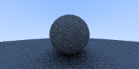Diffuse sphere

Gamma Correction

Our spheres are reflecting 50% of each bounce, so why is our picture so dark? Most image viewers assume images to be “gamma-corrected.” Ours is not. Here’s an explanation of gamma correction from Wikipedia:

Gamma correction, or often simply gamma, is a nonlinear operation used to encode and decode luminance or tristimulus values in video or still image systems.

You can read more about gamma correction here if you feel so compelled.

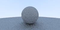
So basically, we need to transform our values before storing them. For a start, we’ll use gamma 2 - which would mean raising the colors to the power of 1/gamma (or.5) - mathematically identical to the square root:

main.cpp:

...

int main() {

	int nx = 200; // Number of horizontal pixels
	int ny = 100; // Number of vertical pixels
	int ns = 10; // Number of samples for each pixel for anti-aliasing
	int maxDepth = 50; // Bounce limit
	std::cout << "P3\n" << nx << " " << ny << "\n255\n"; // P3 signifies ASCII, 255 signifies max color value

	// Create spheres
	hittable *list[2];
	list[0] = new sphere(vec3(0, 0, -1), 0.5);
	list[1] = new sphere(vec3(0, -100.5, -1), 100);
	hittable* world = new hittable_list(list, 2);
	camera cam;

	for (int j = ny - 1; j >= 0; j--) { // Navigate canvas
	    std::cerr << "\rScanlines remaining: " << j << ' ' << std::flush;
		for (int i = 0; i < nx; i++) {
			vec3 col(0, 0, 0);
			for (int s = 0; s < ns; s++) { // Anti-aliasing - get ns samples for each pixel
				double u = (i + random_double(0.0, 1)) / double(nx);
				double v = (j + random_double(0.0, 1)) / double(ny);
				ray r = cam.get_ray(u, v);
				vec3 p = r.point_at_parameter(2.0);
				col += color(r, world, maxDepth);
			}

			col /= double(ns); // Average the color between objects/background
			col = vec3(sqrt(col[0]), sqrt(col[1]), sqrt(col[2]));  // set gamma to 2
			int ir = int(255.99 * col[0]);
			int ig = int(255.99 * col[1]);
			int ib = int(255.99 * col[2]);
			std::cout << ir << " " << ig << " " << ib << "\n";
		}
	}
    std::cerr << "\nDone.\n";
}

Shadow Acne

There’s one small issue left to fix, known as shadow acne. Some of the rays hit the sphere (or any object, really) not at t = 0, but rather at something like t = ±0.0000001 due to floating-point approximation. In that case, we’ll just change our hit detection specs in main.cpp:

if (world.hit(r, 0.001, DBL_MAX, rec)) {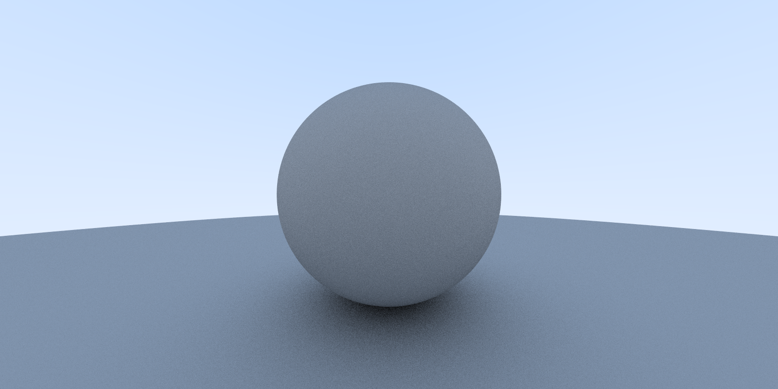

(Mouseover) Fix shadow acne

You can view the images separately, as well. Here’s the one with shadow acne and the one without.

True Lambertian Reflection

Recall that Lambertian reflectance is the “ideal” matte surface - the apparent brightness of a Lambertian surface to an observer is the same regardless of the observer’s angle of view.

Here’s Shirley’s explanation of the implementation of true Lambertian reflectance:

The rejection method presented here produces random points in the unit ball offset along the surface normal. This corresponds to picking directions on the hemisphere with high probability close to the normal, and a lower probability of scattering rays at grazing angles. This distribution scales by the cos3(ϕ) where ϕ is the angle from the normal. This is useful since light arriving at shallow angles spreads over a larger area, and thus has a lower contribution to the final color. However, we are interested in a Lambertian distribution, which has a distribution of cos(ϕ). True Lambertian has the probability higher for ray scattering close to the normal, but the distribution is more uniform. This is achieved by picking points on the surface of the unit sphere, offset along the surface normal. Picking points on the sphere can be achieved by picking points in the unit ball, and then normalizing those.

And our total replacement for random_unit_sphere_coordinate(): (use 3.14 as pi for now, we’ll address it in the next section)

vec3 random_unit_vector() {
    auto a = random_double(0, 2*pi);
    auto z = random_double(-1, 1);
    auto r = sqrt(1 - z*z);
    return vec3(r*cos(a), r*sin(a), z);
}

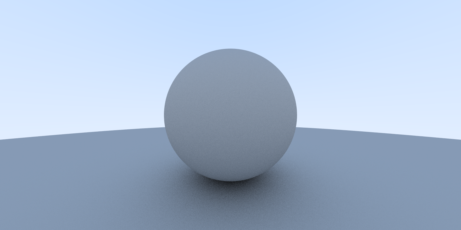
The result:

(Mouseover)True lambertian reflectance

• Lambertian approximation
• True Lambertian

It’s a subtle difference, but a difference nonetheless. Notice that the shadows are not as pronounced and that both spheres are lighter.

These changes are both due to the more uniform scattering toward the normal. For diffuse objects, they appear lighter because more light bounces toward the camera. For shadows, less light bounces straight up.

---

Common Constants and Utilities

You may have noticed in random_unit_vector() that pi is not defined. That’s because in Shirley’s newer edition, he creates a general main header file with some constants and utilities:

#ifndef RTWEEKEND_H
#define RTWEEKEND_H

#include <cmath>
#include <cstdlib>
#include <limits>
#include <memory>


// Usings
using std::shared_ptr;
using std::make_shared;
using std::sqrt;

// Constants
const double infinity = std::numeric_limits<double>::infinity();
const double pi = 3.1415926535897932385;

// Utility Functions
inline double degrees_to_radians(double degrees) {
    return degrees * pi / 180;
}

// Common Headers
#include "ray.h"
#include "vec3.h"

#endif

And uses it in main.cpp:

#include <iostream>
#include <cfloat>


#include "rtweekend.h"


#include "sphere.h"
#include "hittableList.h"
#include "camera.h"
#include "random.h"

vec3 random_unit_vector() {
	auto a = random_double(0, 2*pi);
    auto z = random_double(-1, 1);
    auto r = sqrt(1 - z*z);
    return vec3(r*cos(a), r*sin(a), z);
}

/*
* Assign colors to pixels
*
* Background -
* Linearly blends white and blue depending on the value of y coordinate (Linear Blend/Linear Interpolation/lerp).
* Lerps are always of the form: blended_value = (1-t)*start_value + t*end_value.
* t = 0.0 = White
* t = 1.0 = Blue
* 
* Draw sphere and surface normals
*/
vec3 color(const ray& r, hittable * world, int depth) {
	hit_record rec;

	if (depth <= 0)
        return vec3(0,0,0); // Bounce limit reached - return darkness

	if (world->hit(r, 0.001, infinity, rec)) { 
		vec3 target = rec.p + rec.normal + random_unit_vector(); 
		return 0.5 * color(ray(rec.p, target - rec.p), world, depth-1); // light is absorbed continually by the sphere or reflected into the world.
	}
	else { // background
		vec3 unit_direction = unit_vector(r.direction());
		double t = 0.5 * (unit_direction.y() + 1.0);
		return (1.0 - t) * vec3(1.0, 1.0, 1.0) + t * vec3(0.5, 0.7, 1.0);
	}
}

int main() {

	int nx = 1600; // Number of horizontal pixels
	int ny = 800; // Number of vertical pixels
	int ns = 10; // Number of samples for each pixel for anti-aliasing
	int maxDepth = 50; // Bounce limit

	std::cout << "P3\n" << nx << " " << ny << "\n255\n"; // P3 signifies ASCII, 255 signifies max color value

	// Create spheres
	hittable *list[2];
	list[0] = new sphere(vec3(0, 0, -1), 0.5);
	list[1] = new sphere(vec3(0, -100.5, -1), 100);
	hittable* world = new hittable_list(list, 2);
	camera cam;

	for (int j = ny - 1; j >= 0; j--) { // Navigate canvas
	        std::cerr << "\rScanlines remaining: " << j << ' ' << std::flush;

		for (int i = 0; i < nx; i++) {
			vec3 col(0, 0, 0);
			for (int s = 0; s < ns; s++) { // Anti-aliasing - get ns samples for each pixel
				double u = (i + random_double(0.0, 0.999)) / double(nx);
				double v = (j + random_double(0.0, 0.999)) / double(ny);
				ray r = cam.get_ray(u, v);
				vec3 p = r.point_at_parameter(2.0);
				col += color(r, world, maxDepth);
			}

			col /= double(ns); // Average the color between objects/background
			col = vec3(sqrt(col[0]), sqrt(col[1]), sqrt(col[2]));  // set gamma to 2
			int ir = int(255.99 * col[0]);
			int ig = int(255.99 * col[1]);
			int ib = int(255.99 * col[2]);
			std::cout << ir << " " << ig << " " << ib << "\n";
		}
	}
}

While we’re here making changes, let’s clean things up a bit by:

• Moving random_unit_vector() to vec3.h
• Moving our random number generator to rtweekend.h

---

Metal

Abstract Class for Materials

We’re going to use an abstract material class that encapsulates behavior which will do two things:

• Produce a scattered ray (or absorb the incident ray)
• Determine attenuation (reduction of magnitude) of a scattered ray

material.h:

#ifndef MATERIAL_H
#define MATERIAL_H

class material {
    public:
        virtual bool scatter(
            const ray& r_in, const hit_record& rec, color& attenuation, ray& scattered
        ) const = 0;
};

#endif

Describing Ray-Object Intersections

The hit_record struct in hittable.h is where we’ll be storing whatever information we want about hits. We’ll be adding material to the struct.

hittable.h:

#ifndef HITTABLEH
#define HITTABLEH

#include "ray.h"

class material; // forward declaration

struct hit_record {
	double t; // parameter of the ray that locates the intersection point
	vec3 p; // intersection point
	vec3 normal;
	bool front_face;
	material* material_ptr;

	inline void set_face_normal(const ray& r, const vec3& outward_normal) {
        front_face = dot(r.direction(), outward_normal) < 0;
        normal = front_face ? outward_normal : -outward_normal;
    }
};

/* 
* A class for objects rays can hit.
*/
class hittable {
public: 
	virtual bool hit(const ray& r, double t_min, double t_max, hit_record& rec) const = 0;
};

#endif // !HITTABLEH

When a ray hits a surface, the material pointer within the hit struct will point to the material the object was instantiated with. As such, we’ll have to reference the material within our sphere class to be included with the hit_record.

sphere.h:

#ifndef SPHEREH
#define SPHEREH

#include "hittable.h"

class sphere : public hittable {
public:
	sphere() {}
	sphere(vec3 cen, float r, material* material) : center(cen), radius(r), material_ptr(material) {};
	virtual bool hit(const ray& r, double tmin, double tmax, hit_record& rec) const;
	vec3 center;
	double radius;
	material* material_ptr;
};

bool sphere::hit(const ray& r, double t_min, double t_max, hit_record& rec) const {
	vec3 oc = r.origin() - center; // Vector from center to ray origin
	double a = r.direction().length_squared();
	double halfB = dot(oc, r.direction());
	double c = oc.length_squared() - radius*radius;
	double discriminant = (halfB * halfB) - (a * c);
	if (discriminant > 0.0) {
        auto root = sqrt(discriminant);

		auto temp = (-halfB - root) / a;

		if (temp < t_max && temp > t_min) {
			rec.t = temp;
			rec.p = r.point_at_parameter(rec.t);
			vec3 outward_normal = (rec.p - center) / radius;
            rec.set_face_normal(r, outward_normal);
			rec.material_ptr = material_ptr;
			return true;
		}
		temp = (-halfB + root) / a;
		if (temp < t_max && temp > t_min) {
			rec.t = temp;
			rec.p = r.point_at_parameter(rec.t);
			vec3 outward_normal = (rec.p - center) / radius;
            rec.set_face_normal(r, outward_normal);
			rec.material_ptr = material_ptr;
			return true;
		}
	}
	return false;
}

#endif // !SPHEREH

Light Scatter

The Lambertian material we modeled previously would either scatter and attenuate by its reflectance R, or scatter with no attenuation but absorb 1 - R of rays, or somewhere in between. This is represented in code as follows:

material.h

...
class lambertian : public material {
    public:
        lambertian(const vec3& a) : albedo(a){};
        virtual bool scatter(const ray& ray_in,
                            const hit_record& rec,
                            vec3& attenuation,
                            ray& scattered) const {
            vec3 scatter_direction = rec.p + rec.normal + random_unit_vector();
            scattered = ray(rec.p, target - rec.p);
            attenuation = albedo;
            return true;
        }
    vec3 albedo; // reflectivity

};
...

Metal Reflection

Metal is definitely NOT Lambertian - here’s a simple sketch depecting a general mirrored reflection:

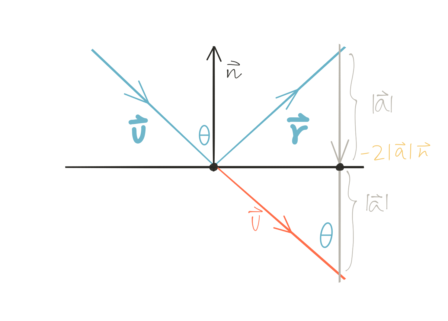Metal Reflection (source)

$$ \vec r = \vec v - (-2 * \vert \vec a\vert * \vec n) $$ where $$ \vert \vec a\vert = \vert \vec v\vert * cos(\theta) $$ since $$ dot(\vec v, \vec n) = \vert \vec v\vert \vert \vec n\vert cos(\pi - \theta) = -\vert \vec v\vert cos(\theta) $$ that means $$ \vert \vec a\vert = -dot(\vec v, \vec n) $$ and $$ \vec r = \vec v - (2 * dot(\vec v, \vec n) * \vec n) $$

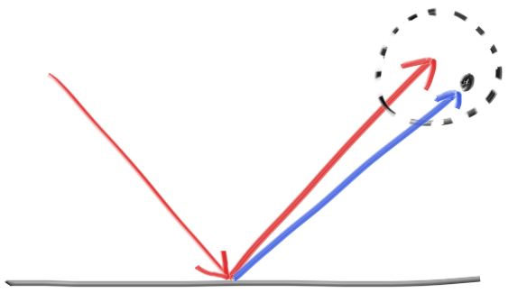
In other words, the reflected ray is v + 2a. N is a unit vector, but that might not be the case for v. Also, because v points inward, we’re going have to flip it by negating it. This yields the following formula:

vec3 reflect(const vec3& v, const vec3& n){
    return v - 2*dot(v,n)*n;
}

We can go ahead and incorporate this formula into our metal material:

material.h

vec3 reflect(const vec3& v, const vec3& n){
    return v - 2*dot(v,n)*n; // v enters the hittable, which is why subtraction is required.
}

class material {
    public:
    virtual bool scatter(const ray& ray_in, const hit_record& rec, vec3& attenuation, ray& scattered) const = 0;
};

// Matte surface
// Light that reflects off a diffuse surface has its direction randomized.
// Light may also be absorbed. See Diffuse.png for illustration and detailed description
class lambertian : public material {
    public:
        lambertian(const vec3& a) : albedo(a){};
        virtual bool scatter(const ray& ray_in, const hit_record& rec, vec3& attenuation, ray& scattered) const {
            vec3 target = rec.p + rec.normal + random_unit_sphere_coordinate();
            scattered = ray(rec.p, target - rec.p);
            attenuation = albedo;
            return true;
        }
    vec3 albedo; // reflectivity

};

class metal : public material {
    public:
        metal(const vec3& a) : albedo(a) {}
        virtual bool scatter(const ray& ray_in, const hit_record& rec, vec3& attenuation, ray& scattered) const {
        vec3 reflected = reflect(unit_vector(ray_in.direction()), rec.normal);
        scattered = ray(rec.p, reflected);
        attenuation = albedo;
        return dot(scattered.direction(), rec.normal) > 0.0;
    }

    vec3 albedo;
};

And of course, we’re going to need to update our color() function to use our new material: main.cpp:

vec3 color(const ray& r, hittable *world, int depth) {
    hit_record rec;

    if (depth <= 0) {
        return vec3(0,0,0);
    }  
    if (world->hit(r, 0.001, DBL_MAX, rec)) {
        ray scattered;
        vec3 attenuation;
		// Scatter formulas vary based on material
        if (rec.material_ptr->scatter(r, rec, attenuation, scattered)) {
            return attenuation*color(scattered, world, depth-1);
        }
        else {
            return vec3(0,0,0);
        }
    }
    else {
        vec3 unit_direction = unit_vector(r.direction());
        double t = 0.5*(unit_direction.y() + 1.0);
        return (1.0-t)*vec3(1.0, 1.0, 1.0) + t*vec3(0.5, 0.7, 1.0);
    }
}

Adding Metal Spheres to the Scene

Now that we’ve got some shiny new spheres, let’s add ‘em to the scene, render ‘em, and check ‘em out: main.cpp:

int main {
	...

	hittable *list[4];
		hittable *list[4];
    	list[0] = new sphere(vec3(0,0,-1), 0.5, new lambertian(vec3(0.8, 0.3, 0.3)));
		list[1] = new sphere(vec3(0,-100.5,-1), 100, new lambertian(vec3(0.8, 0.8, 0.0)));
		list[2] = new sphere(vec3(1,0,-1), 0.5, new metal(vec3(0.8, 0.6, 0.2)));
		list[3] = new sphere(vec3(-1,0,-1), 0.5, new metal(vec3(0.8, 0.8, 0.8)));
		hittable *world = new hittable_list(list,4);

		camera cam(lookFrom, lookAt, vec3(0,1,0), 20,double(nx)/double(ny), aperture, distToFocus);	

		auto start = std::chrono::high_resolution_clock::now();


		for (int j = ny - 1; j >= 0; j--) { // Navigate canvas

		...

You’ll get something like this:

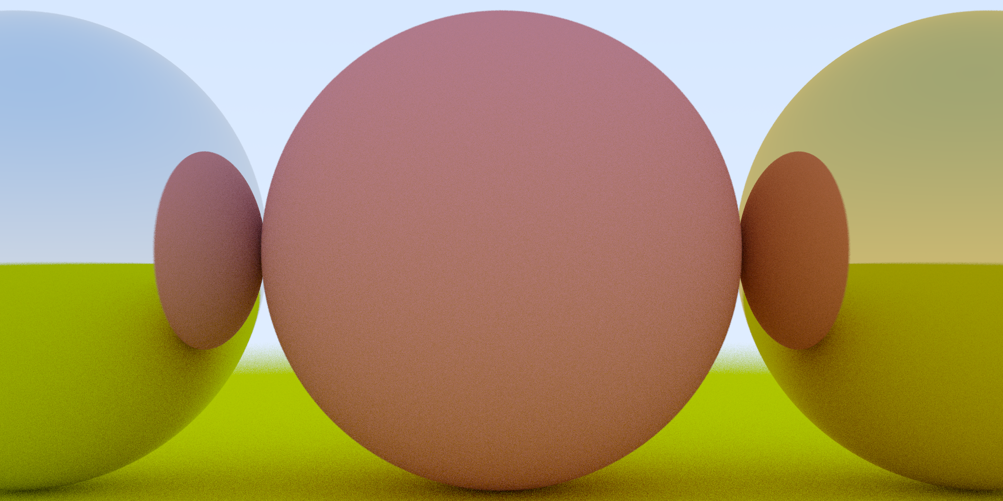Metal and Lambertian spheres

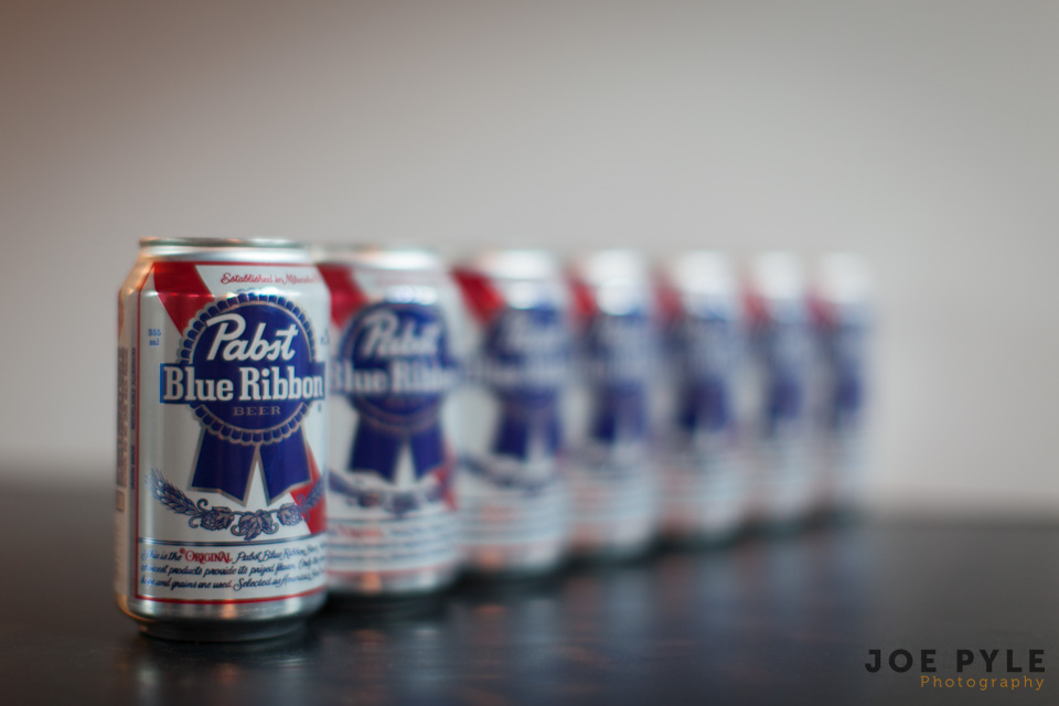
Feel free to mess around with the color, positioning, and material, as well:

Your new album cover

Fuzzy Metal

In addition to perfectly polished metal spheres, we can simulate rough metal as well, with some “fuzziness.” To do so, we just need to append a random vector to the reflected rays:

Generating fuzzy reflections (source)

The larger the sphere, the fuzzier the reflections will be. If the sphere is too large, we may scatter below the surface of an object. If that happens, we can just have the surface absorb those rays.

material.h:

class metal : public material {
    public:
        metal(const vec3& a, double f) : albedo(a) {
			if (f<1) fuzz = f; else fuzz = 1;
        }
        virtual bool scatter(const ray& ray_in, const hit_record& rec, vec3& attenuation, ray& scattered) const {
        vec3 reflected = reflect(unit_vector(ray_in.direction()), rec.normal);
        scattered = ray(rec.p, reflected);
        attenuation = albedo;
        return dot(scattered.direction(), rec.normal) > 0.0;
    }

    vec3 albedo;
	double fuzz;
};

(Mouseover) Fuzziness from left to right: .5, 0, and 1

• No fuzz
• Fuzz

---

Dielectrics

Dielectrics are materials like glass. When a light ray hits one, the ray splits into a reflected ray and a refracted ray. In this path tracer, we’ll be randomly choosing which ray to simulate, only generating one ray per interaction.

Refraction

Refraction is the deflection of a ray from a straight path due to passing obliquely from one medium to another.

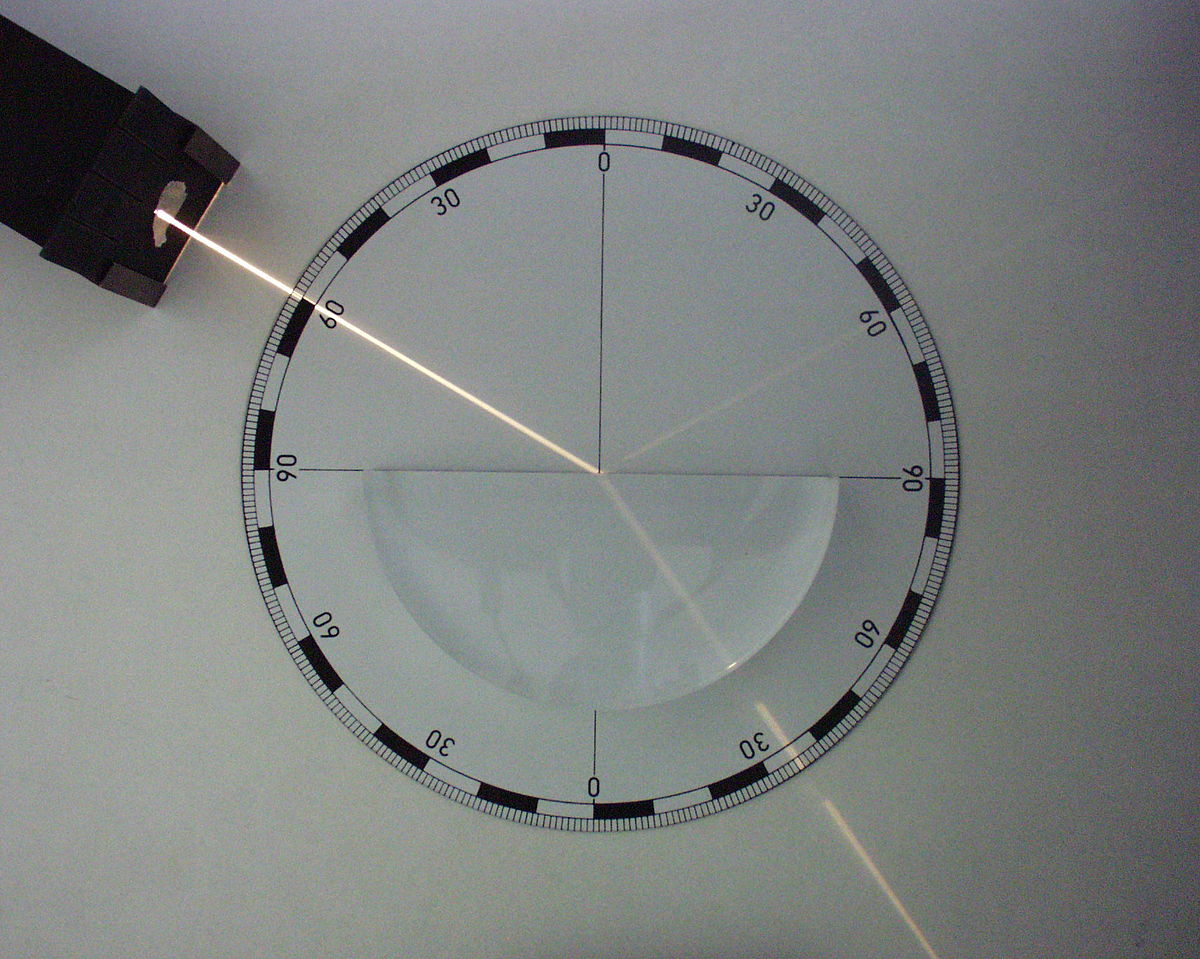Notice both the reflected beam (top right) and the refracted beam (bottom right) (source)

The refractive index describes the angle that light propagates through different mediums and is defined as:

\[n={\frac {c}{v}}\]

where c is the speed of light in a vacuum and v is the speed of light in the medium.

For reference, here are some refractive indices:

Material	Refractive Index
Vacuum	1
Air	1.000293
Carbon Dioxide	1.001
Ice	1.31
Water	1.333
Kerosene	1.39
Vegetable Oil	1.47
Window Glass	1.52
Amber	1.55
Diamond	2.417
Germanium	4.05

Snell’s Law

Snell’s law states that the ratio of the sines of the angles of incidence and refraction is equivalent to the ratio of phase velocities in the two media, or equivalent to the reciprocal of the ratio of the indices of refraction:

\[{\frac {\sin \theta _{2}}{\sin \theta _{1}}}={\frac {v_{2}}{v_{1}}}={\frac {n_{1}}{n_{2}}}\]

with each θ as the angle measured from the normal of the boundary, v as the velocity of light in the respective medium, n as the refractive index (which is unitless) of the respective medium.

If we render a dielectric object with ref_index in a vacuum, (since the refractive index is 1 in a vacuum) we get this:

\[\frac {n_{1}}{n_{2}} = \frac {1}{ref\_index}\]

and when the ray shoots back out into the vacuum:

\[\frac {n_{1}}{n_{2}} = {ref\_index}\]

Total Internal Reflection

Total internal reflection is an optical phenomenon that occurs when light travels from a medium with a higher refractive index to a lower one, and the angle of incidence is greater than a certain angle (known as the “critical angle”).

Calculating the Refraction Vector

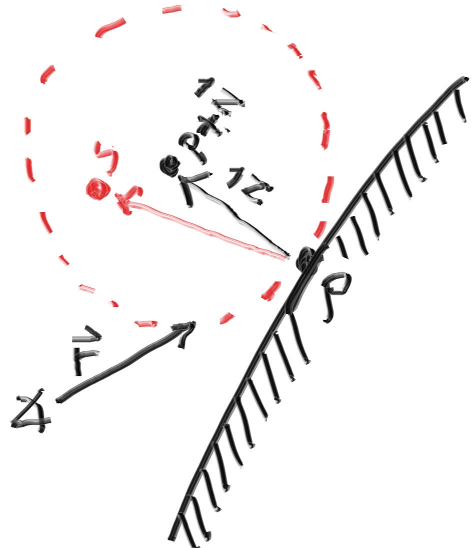
Now that we’re familiar with the components of refraction, we can calculate the refraction vector geometrically.

We can model the relationships of the vectors with a unit circle to make things easier.

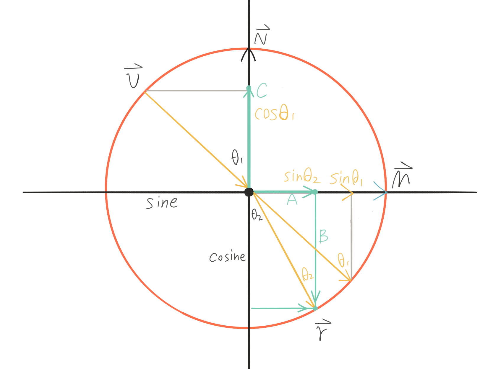(source)

\[\vec r = \vec A + \vec B\]

We’ll project $\vec r$ onto $\vec M$ to get $\vec A$:

\[\vec A = sin\theta_{2} \cdot \vec M\]

Similarly, we’ll project $\vec r$ onto $- \vec N$ to get $\vec B$:

\[\vec B = cos\theta_{2} \cdot -\vec N\]

We’ll define $\vec M$ as perpendicular($\bot$) to $\vec N$:

\[\vec M = Normalize(\vec C + \vec v) = \frac {(\vec C + \vec v)}{sin\theta_{1}}\]

And we’ll project $\vec r$ onto $- \vec N$ to get $\vec C$:

\[\vec C = cos\theta_{1} \cdot \vec N\]

So, with terms expanded, we go from:

\[\vec r = \vec A + \vec B\]

to:

\[\vec r = sin\theta_{2} \cdot \vec M - cos\theta_{2} \cdot \vec N\]

If we expand and re-arrange the equation, we’ll end up with this:

\[\vec r = \frac {n_{1}}{n_{2}} \cdot (\vec v + cos\theta_{1} \cdot \vec N) - cos\theta_{2} \cdot \vec N\]

After normalizing incidence ray direction $\vec v$ , we can calculate $cos\theta_{1}$ by $dot(\vec v, \vec n) = \vert \vec v\vert \vert \vec n\vert cos\theta_{1} = cos\theta_{1}$.

Since Snell’s law can also be interpreted as:

\[sin\theta_{2} = \frac {n_{1}}{n_{2}} \cdot sin\theta_{1},\] \[cos^2\theta_{2} = 1 - sin^2\theta_{2} = 1 - \frac {(n_1)^2}{(n_2)^2} \cdot sin^2\theta_{1} = 1 - \frac {n_{1}^2}{n_{2}^2} \cdot (1 - cos^2\theta_{1}) = 1 - \frac {n_{1}^2}{n_{2}^2} \cdot (1 - dot(\vec v, \vec n))\]

and the equation can be written as:

\[\vec r = \frac {n_{1}}{n_{2}} \cdot (\vec v - dot(\vec v, \vec n) \cdot \vec N) - \sqrt{1 - \frac {n_{1}^2}{n_{2}^2} \cdot (1 - dot(\vec v, \vec n))} \cdot \vec N\]

Which means that:

\[cos^2\theta_{2} = 1 - \frac {n_{1}^2}{n_{2}^2} \cdot (1 - dot(\vec v, \vec n))\]

is the discriminant.

Discriminant	Ray Behavior
$<0$	Total internal reflection
$=0$	Boundary of total reflection - no resultant ray
$>0$	Refracted ray $\vec r$

Coding the Refraction Vector

• $\frac {n_{1}}{n_{2}}$ is n1_over_n2
• v is the incidence ray
• n is the surface normal
• refracted is the refracted ray’s direction

bool refract(const vec3& v, const vec3& n, float n1_over_n2, vec3& refracted) {
    vec3 uv = unit_vector(v);
    float dt = dot(uv, n);
    float discriminat = 1.0 - ni_over_nt * ni_over_nt * (1-dt*dt);
    if(discriminat > 0){
        refracted = ni_over_nt * (uv-n*dt) - n*sqrt(discriminat);
        return true;
    }
    else
        return false; // no refracted ray
}

Dielectric Reflections

When light strikes a dielectric object, both reflection and refraction may occur. Looking at a puddle at a sharp enough angle makes it look almost like a mirror!

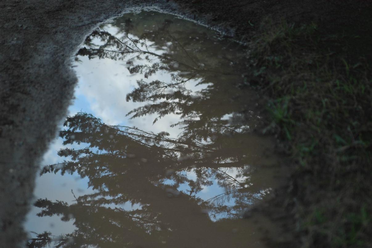
For low-precision applications that don’t involve polarized light, Schlick’s approximation will serve our purposes just fine, rather than computing the effective reflection coefficient for every angle.

Schlick’s model states that the specular reflection coefficient can be approximated by:

\(R(\theta_{1})=R_{0}+(1-R_{0})(1-\cos \theta_{1} )^{5}\) \(R_{0}=\left({\frac {n_{1}-n_{2}}{n_{1}+n_{2}}}\right)^{2}\)

• $\theta_1$ is the incident angle.
• $n_1$ and $n_2$ are the refractive indices of the two media.
• $R_0$ is the reflection coefficient for light incoming parallel to the normal.

The refractive index of air(1.000293) is often approximated as 1.

\[\frac {n_{1}}{n_{2}} = \frac {1}{n_{dielectric}} \Rightarrow {n_{dielectric}} = \frac {n_{2}}{n_{1}}\] \[cos\theta_{1} = dot(\vec v, \vec n)\]

We can add Schlick’s approximation to material.h

material.h:

float schlick(float cosine, float ref_idx) {
    float r0 = (1 - ref_index) / (1 + ref_index); // ref_index = n2/n1
    r0 = r0 * r0;
    return r0 + (1 - r0) * pow((1 - cosine), 5);
}

If the incident ray produces a refraction ray (which we can check by seeing if refract() returns true), we are going to calculate the reflective coefficient reflect_probability. Otherwise, the ray exhibits total internal reflection and the reflective coefficient should be 1.

We do this by getting whichever value is smaller between:

• the dot product of flipped unit incident ray and the normal of the hit point OR
• 1.0 (Total internal reflection)

You may be wondering how we are to represent the refraction and reflection of light if we can only pick one scattered ray. The answer is multi-sampling - averaging the color between samples that may have been reflected or refracted.

To get an accurate result, we’ll use our random number generator. We’ll generate a number between 0.0 and 1.0. If the resulting number is smaller than the reflective coefficient, the ray will be reflected. Otherwise, it will be refracted.

We can now bundle everything up into our dielectric material’s scatter() method:

material.h:

...

class dielectric : public material {
    public:
        dielectric(vec3 a, double ri) : albedo(a), ref_idx(ri) {}

        virtual bool scatter(
            const ray& r_in, const hit_record& rec, vec3& attenuation, ray& scattered
        ) const {

            attenuation = albedo; // color

            double n1_over_n2 = (rec.front_face) ? (1.0 / ref_idx) : (ref_idx);

            vec3 unit_direction = unit_vector(r_in.direction());
            
            double cosine = dot(-unit_direction, rec.normal);
            double reflect_random = random_double(0,1);
            double reflect_probability;

            vec3 refracted;
            vec3 reflected;

			// refracted ray exists
            if (refract(unit_direction, rec.normal, n1_over_n2, refracted)) {
                reflect_probability = schlick(cosine, ref_idx);

                if (reflect_random < reflect_probability) {
                    vec3 reflected = reflect(unit_direction, rec.normal);
                    scattered = ray(rec.p, reflected);
                    return true;
                }
                scattered = ray(rec.p, refracted);
                return true;
            }

            else {
                reflected = reflect(unit_direction, rec.normal);
                scattered = ray(rec.p, reflected);
                return true;
            }
        }
    public:
        double ref_idx;
        vec3 albedo;
};

(Mouseover) Implementation of Fresnel reflections

• No fresnel
• Fresnel

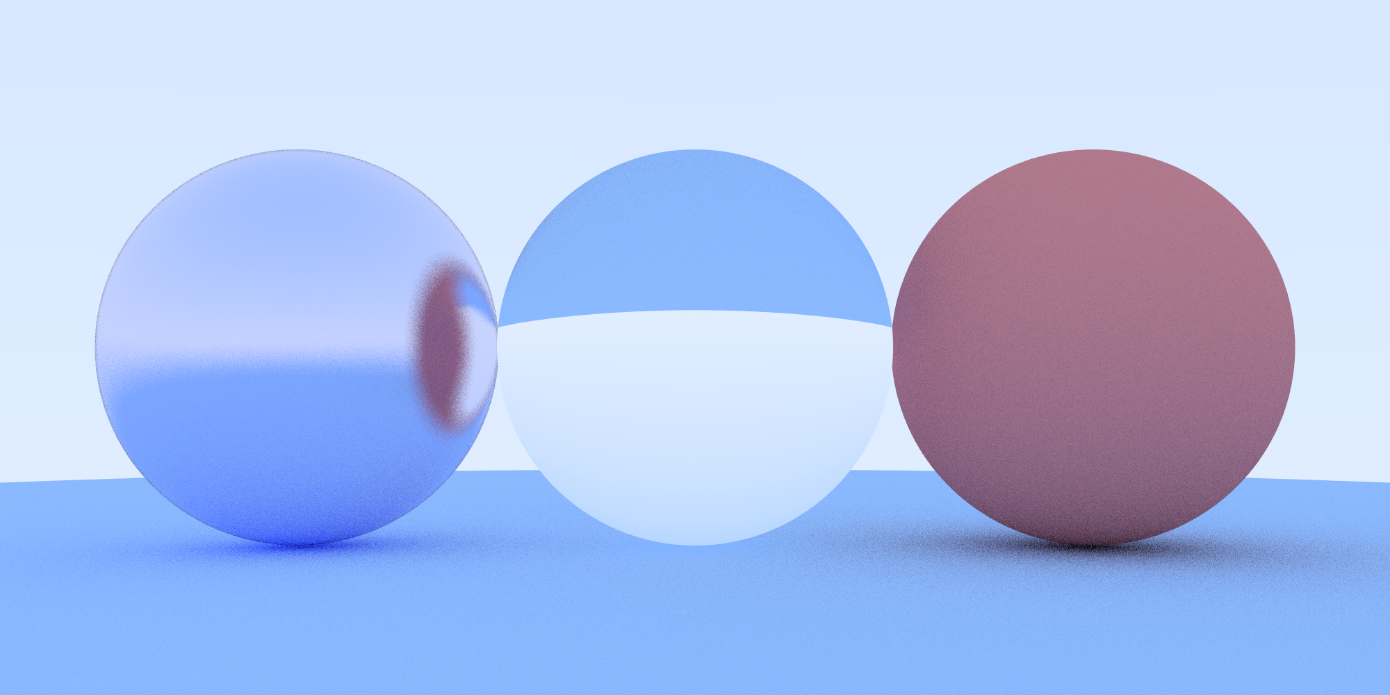
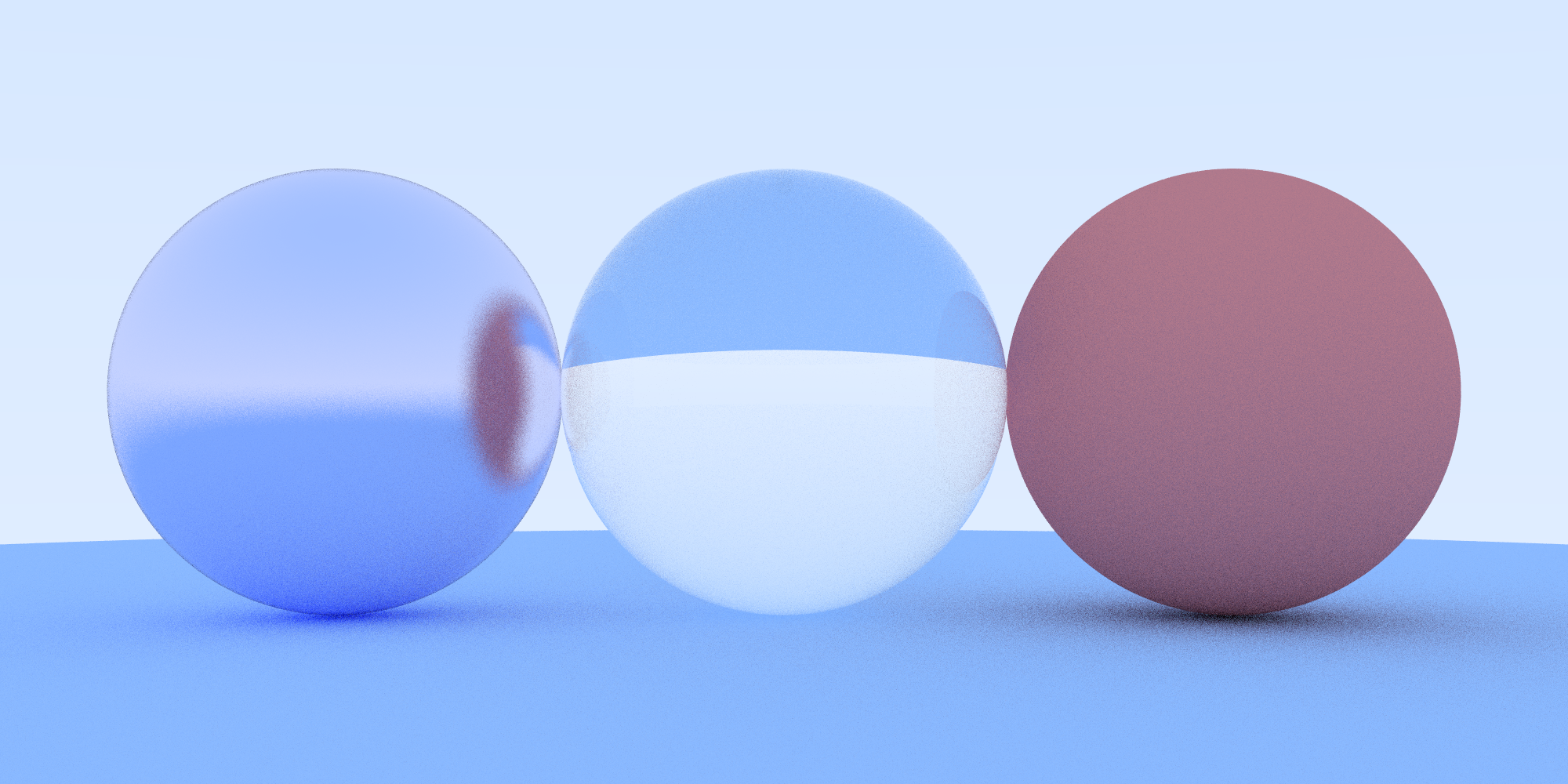
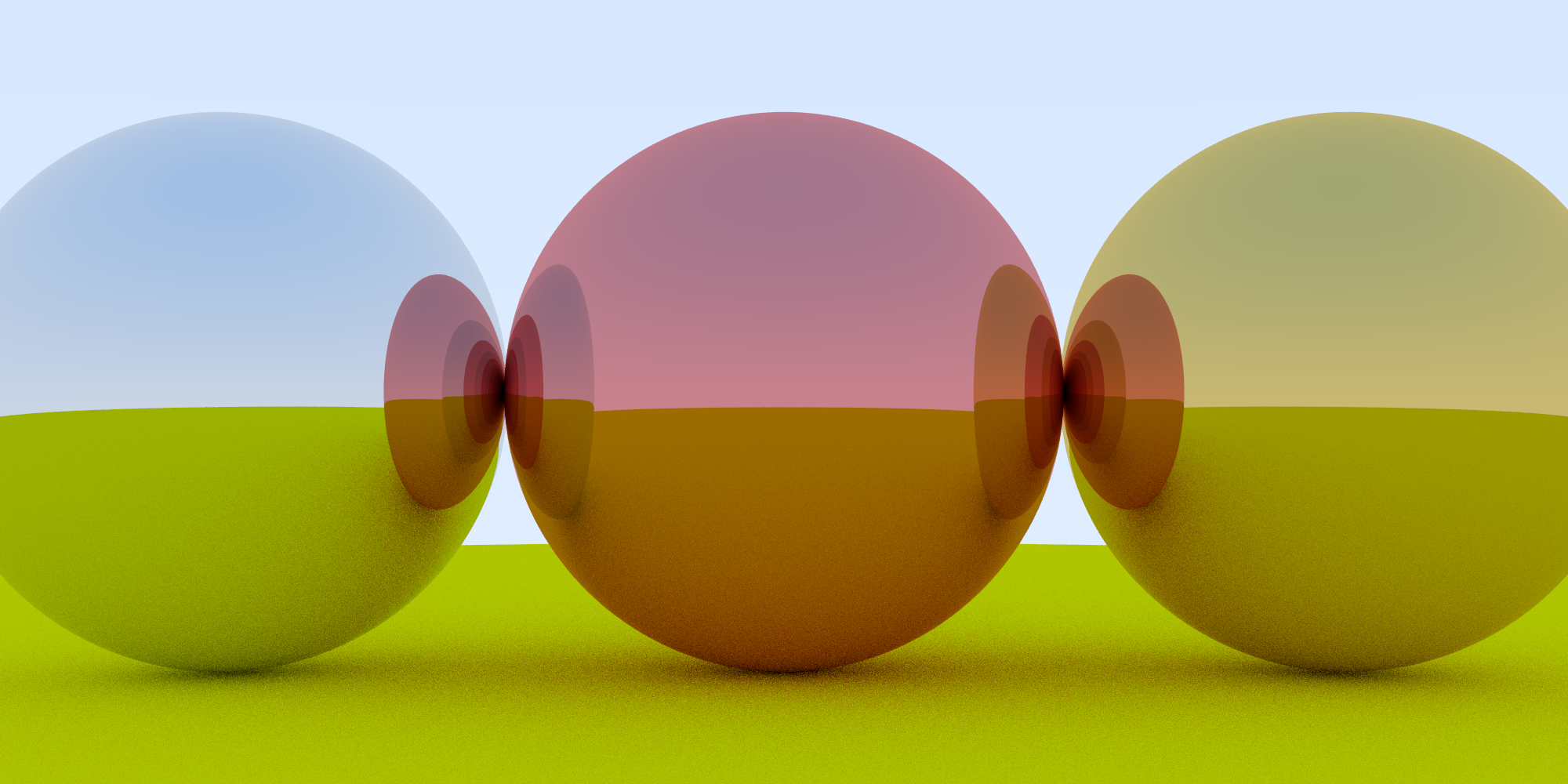
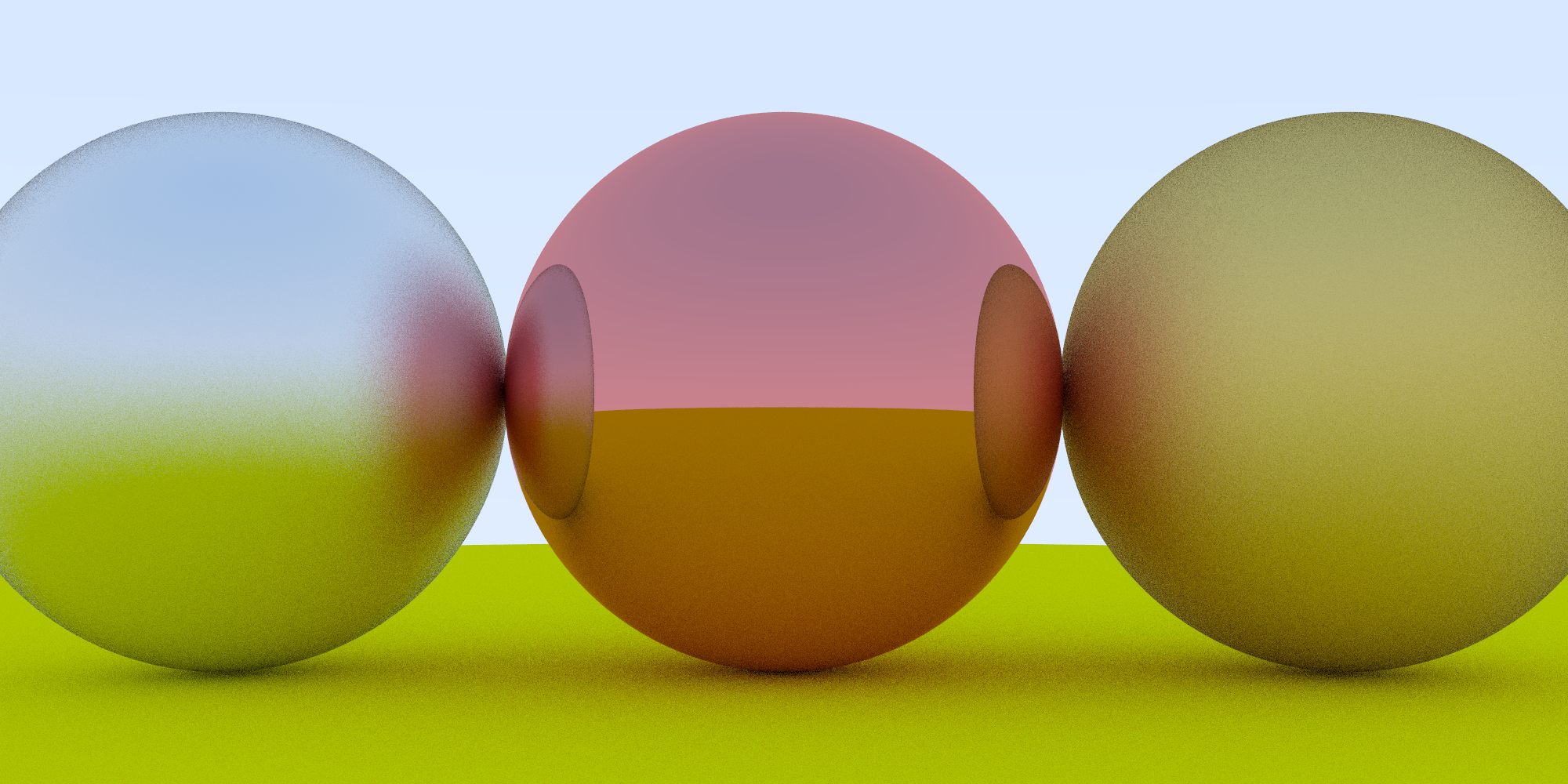
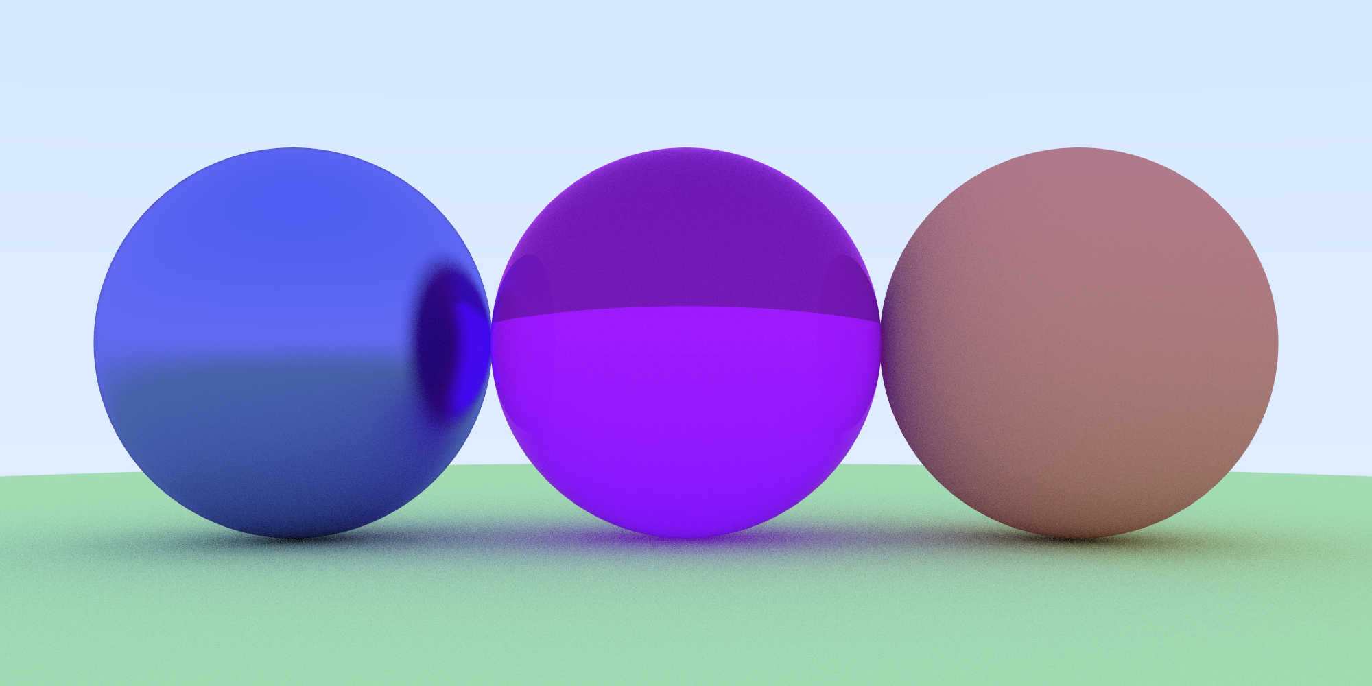
Hollow Dielectric Spheres

Bonus fun fact! We can create a hollow glass sphere by creating a smaller sphere with a negative radius inside our existing sphere! The geometry is unaffected, but the normal points inward.

(Mouseover) Hollow dielectric sphere

• Solid
• Hollow

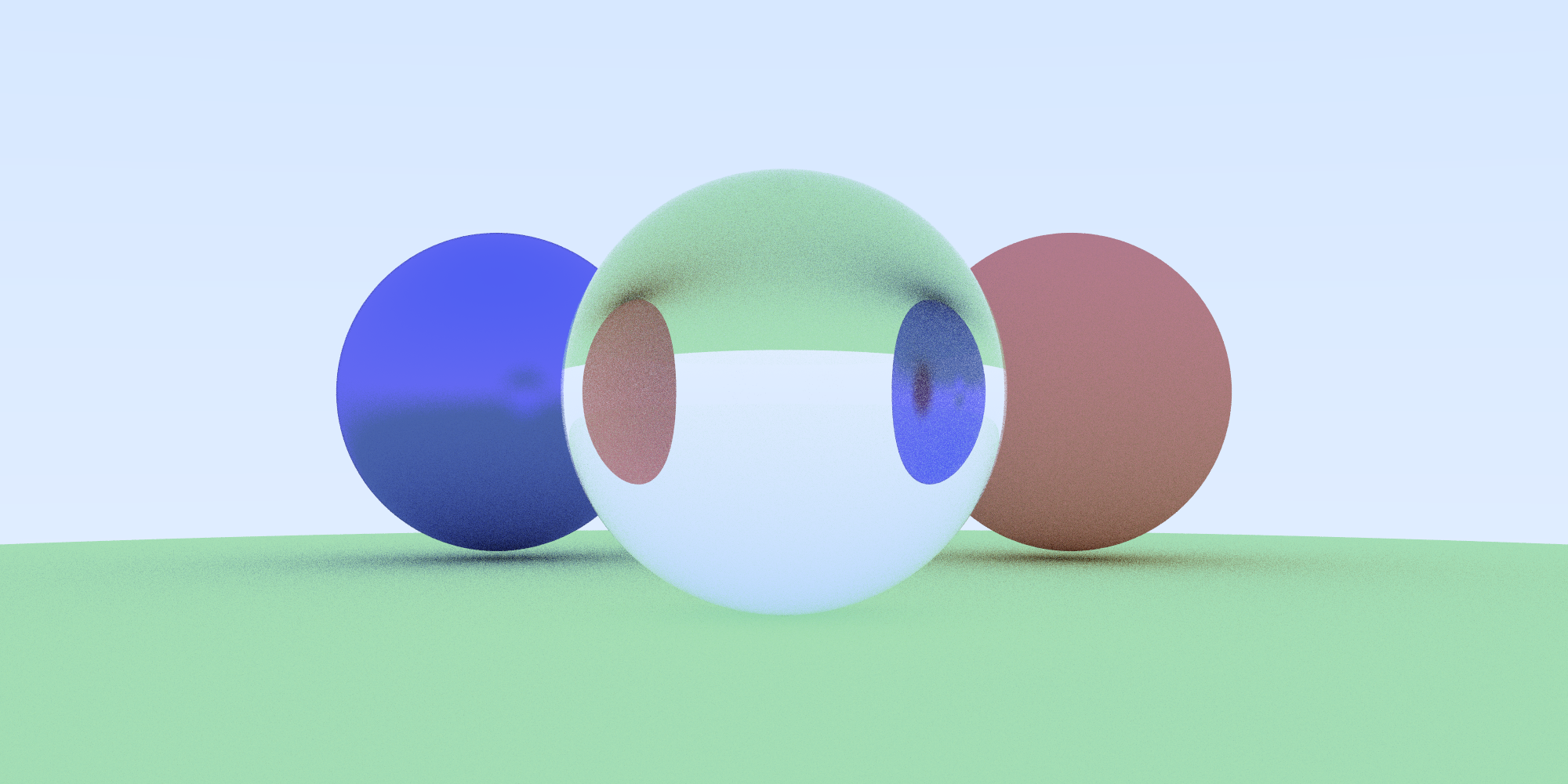
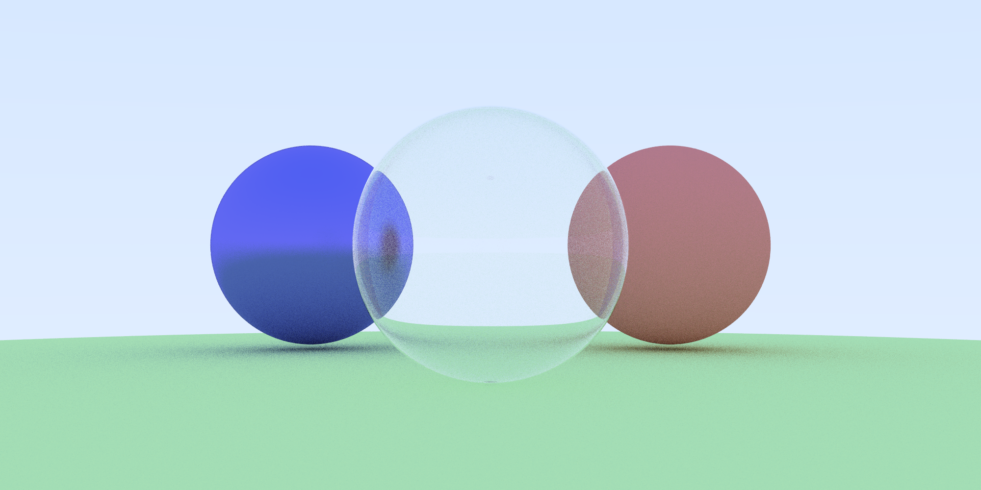
And of course, you can change the color of your pretty new dielectric sphere if you please.

---

Camera Modeling

Up until now, we’ve been using a very simple camera (though I have changed framing a little bit for illustrating certain renders). Our simple camera was described way back in chapter 4 of Shirley’s book, and it had fixed world position at the origin (0, 0, 0), a fixed image plane (or near-clipping plane) size, and the plane was position at (0, 0, -1), effectively setting our sights along the negative z-axis.

camera.h:

#ifndef CAMERAH
#define CAMERAH

#include "ray.h"

class camera {
public:

	// The values below are derived from making the "camera" / ray origin coordinates(0, 0, 0) relative to the canvas.
	camera() {
		lower_left_corner = vec3(-2.0, -1.0, -1.0);
		horizontal = vec3(4.0, 0.0, 0.0);
		vertical = vec3(0.0, 2.0, 0.0);
		origin = vec3(0.0, 0.0, 0.0);
	}
	ray get_ray(double u, double v) { return ray(origin, lower_left_corner + u * horizontal + v * vertical - origin); }

	vec3 origin;
	vec3 lower_left_corner;
	vec3 horizontal;
	vec3 vertical;
};

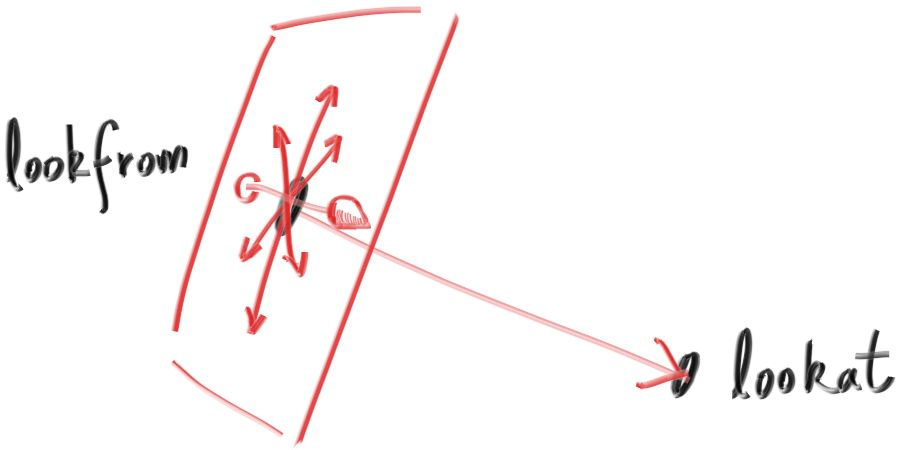
#endif // !CAMERAH

We’re going to expand the capability of the camera and make it more flexible by defining a few different variables:

• Camera position look_from
• Camera objective look_at
• Vector describing which way is “up” vup
• Vertical field-of-view vfov
• Image plane aspect ratio aspect_ratio
• Camera lens size aperture
• Image plane to camera distance focus_distance

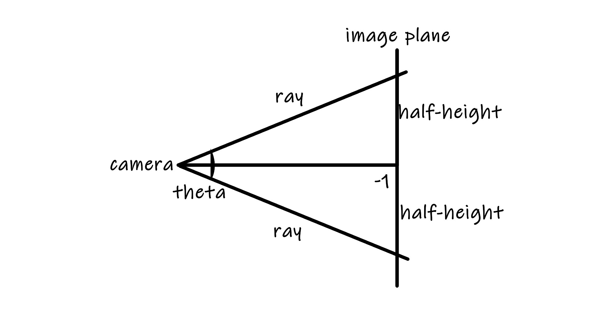
If the angle of the camera lens is theta, we can see that half_height = tan(theta/2).

\[tan(\frac {\theta}{2}) = \frac{opposite}{adjacent} = \frac {half\_height}{1}\]

theta is the vertical field of view vfov. For the convenience of calculation, we can convert theta to radians and define it as vfov * pi / 180.

Keeping other camera settings the same, we can rewrite our camera: camera.h

...
lower_left_corner(-half_width, -half_height,-1.0);
horizontal(2*half_width, 0.0, 0.0); // horizontal range
vertical(0.0, 2*half_height, 0.0);  // vertical range
origin = (0,0,0);
...

In world space(three dimensions), the vectors

\[e1 = (1,0,0),\] \[e2 = (0,1,0),\] \[e3 = (0,0,1)\]

form the standard basis.

The standard basis (for a Euclidean space) is an orthonormal basis, where the relevant inner product is the dot product of vectors. Put simply, this means the vectors are orthogonal: at right angles to each other; and normal: all of the same length 1.

All vectors (x,y,z) in world space can be expressed as a sum of the scaled basis vectors.

\[{\displaystyle (x,y,z)=xe_{1}+ye_{2}+ze_{3}}\]

Every vector $a$ in three dimensions is a linear combination of the standard basis vectors $i$, $j$, and $k$.

Therefore, the previous camera code should be revised to

camera.h

lower_left_corner= origin - half_width * e1 - half_height * e2 - e3
horizontal = 2 * half_width * e1
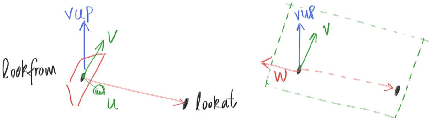
vertical = 2 *half_height * e2

However, if we want to move our “camera” to position look_from pointing to look_at, we have to build a new orthonormal basis for camera space with vectors u, v, and w:

w = unit_vector(lookfrom - lookat) // similar to the Z axis
u = unit_vector(cross(vup, w)) // similar to the X axis
v = cross(w, u) // similar to the Y axis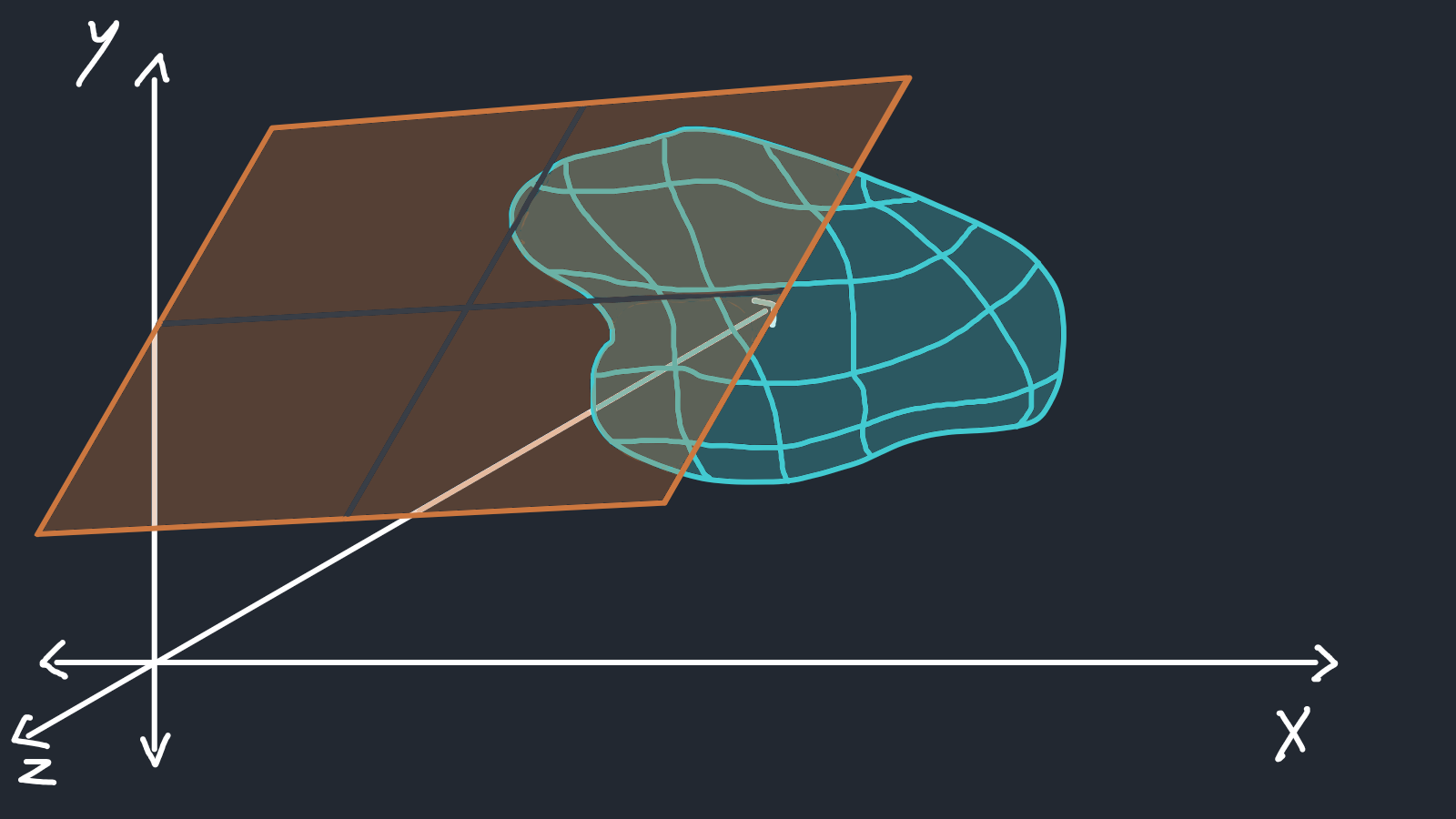

The vup vector describes which direction is up for the camera. You can also think of this as tilt in any (x,y,z).

vup (0,1,0)

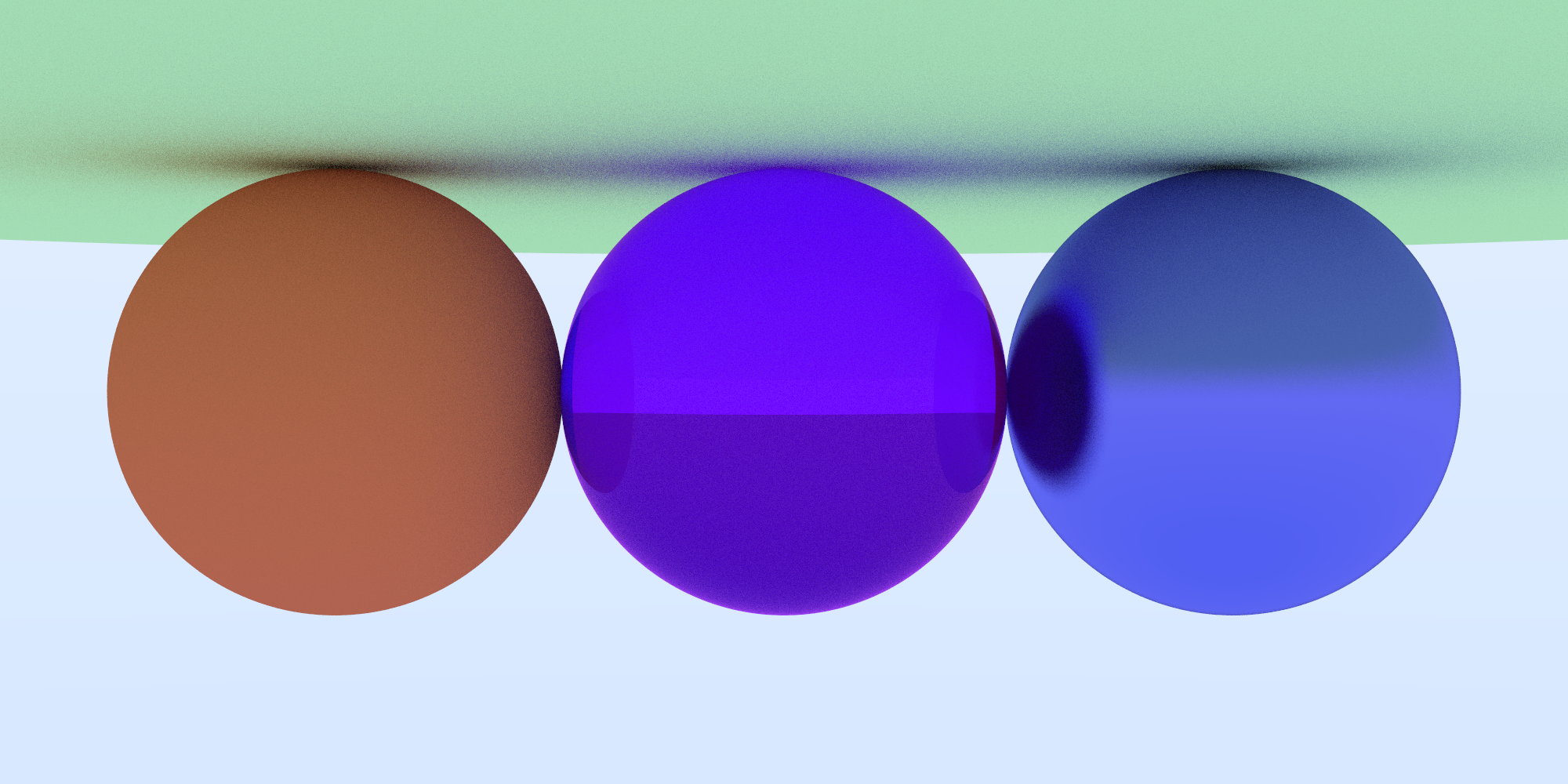vup (0,-1,0)

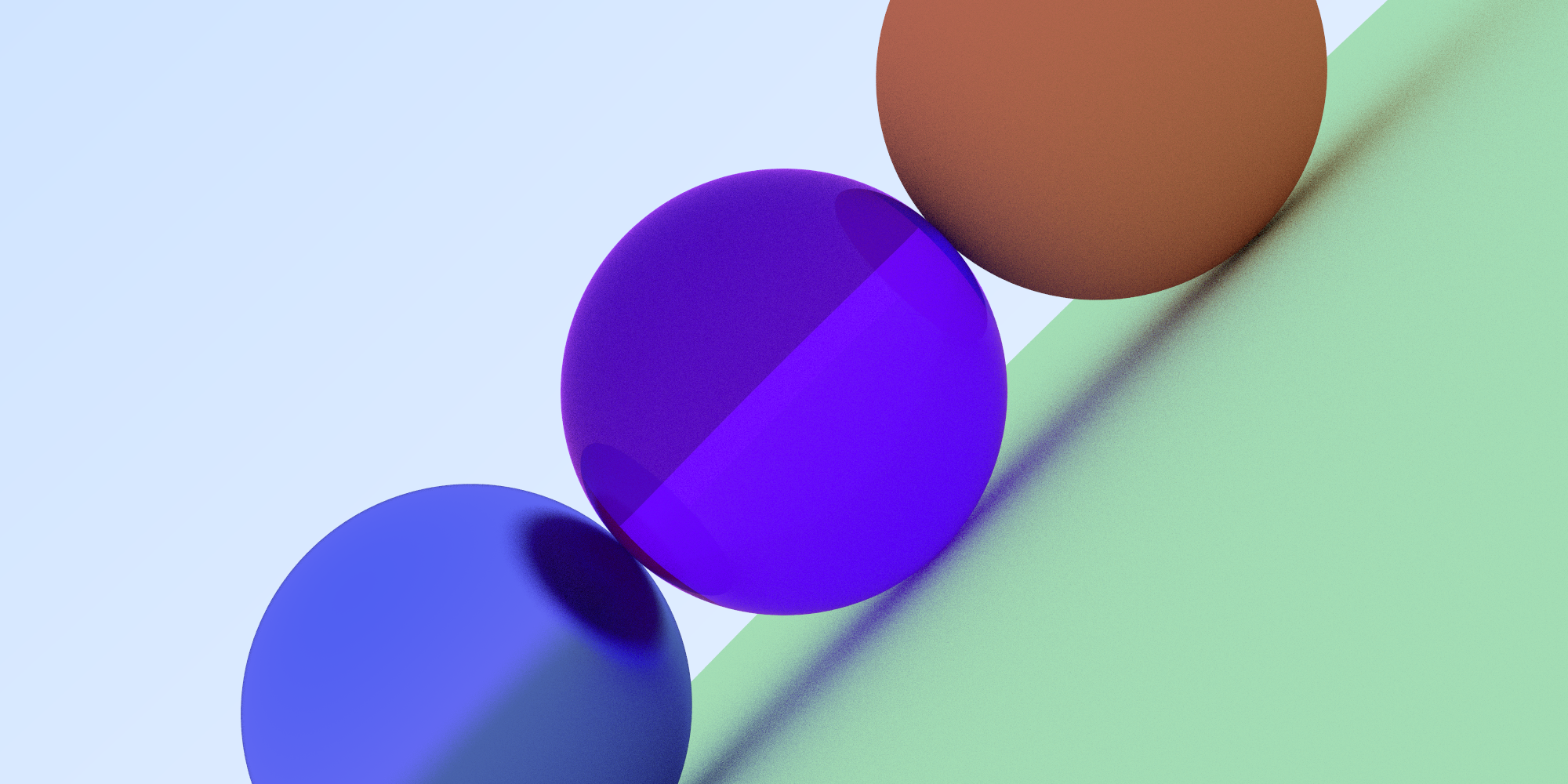vup (1,1,0)

class camera {
public:
    camera(vec3 look_from, vec3 look_at, vec3 vup, float vfov, float aspect_ratio) {
        vec3 u, v, w;

        float theta = vfov*pi/180;
        float half_height = tan(theta/2);
        float half_width = aspect_ratio * half_height;
        origin = lookfrom;

        w = unit_vector(look_from - look_at);
        u = unit_vector(cross(vup, w));
        v = cross(w, u);

        lower_left_corner = origin - half_width*u - half_height*v -w;
        horizontal = 2*half_width*u;
        vertical = 2*half_height*v;
    }
    ray get_ray(float s, float t) {return ray(origin, lower_left_corner + s*horizontal + t*vertical - origin);}

    vec3 lower_left_corner;
    vec3 horizontal;
    vec3 vertical;
    vec3 origin;
};

---

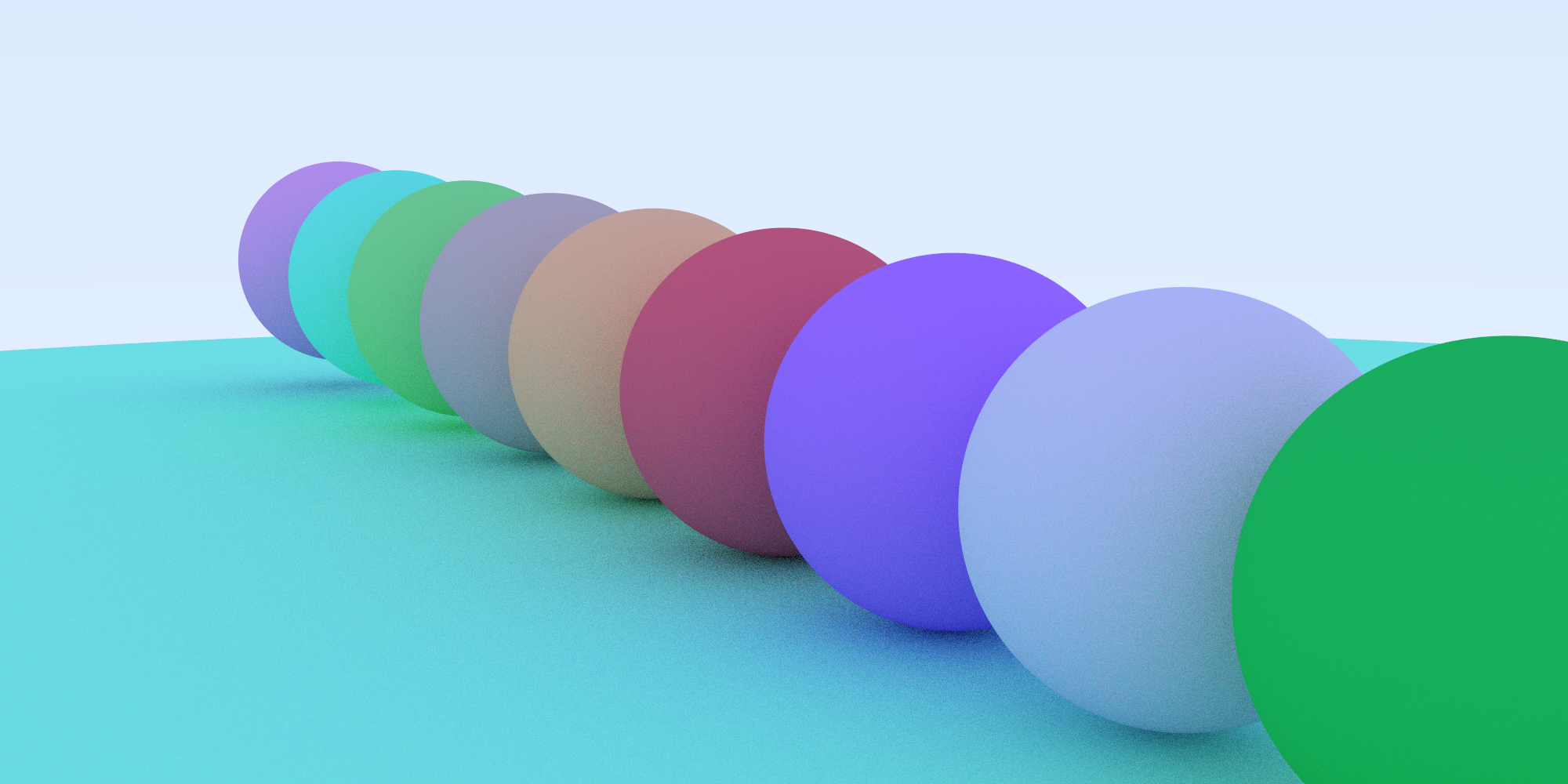
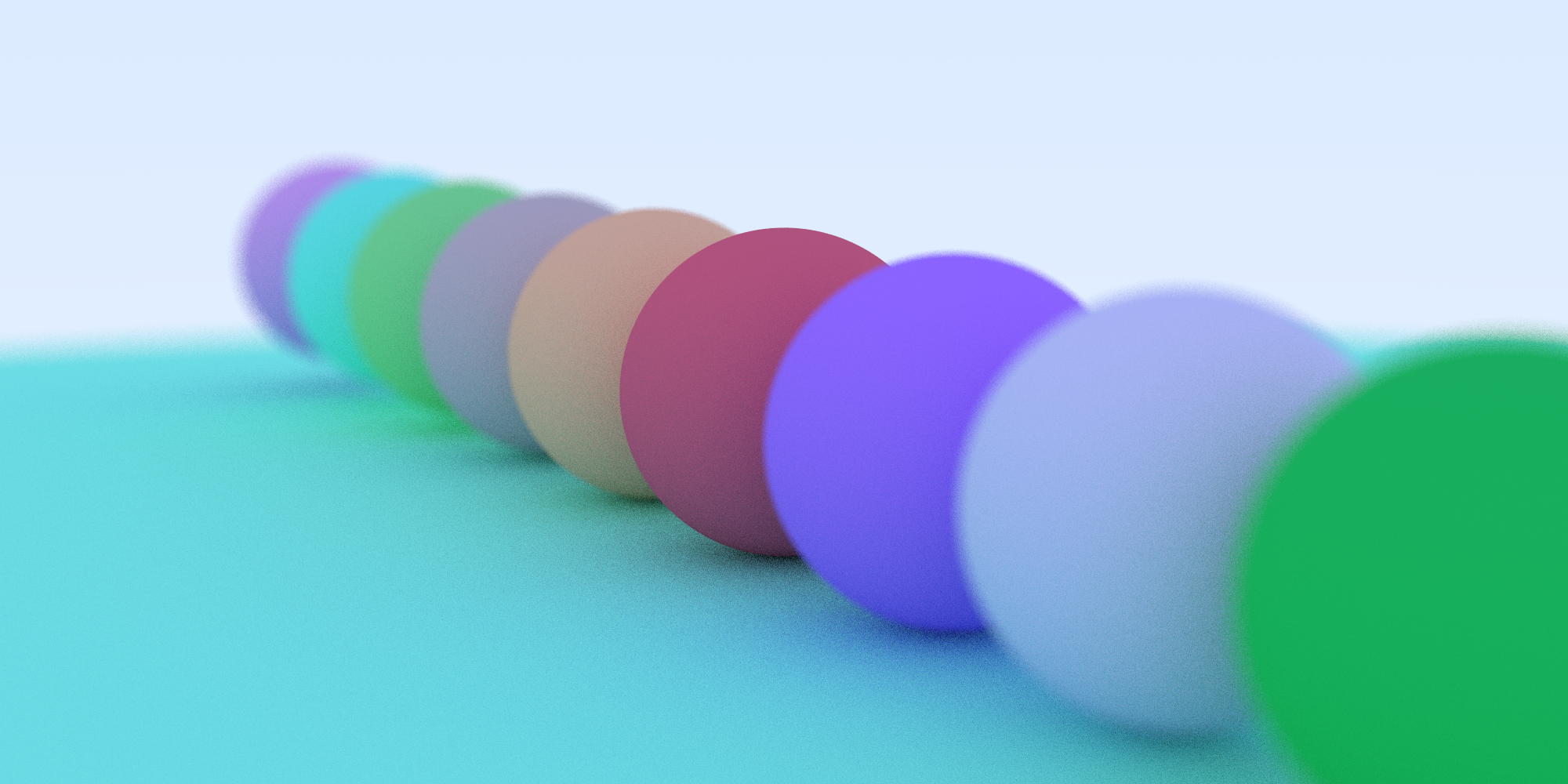
Depth of Field

Depth of field! If you have eyes that kind of work, you’re familiar with it. You can read more about DOF at Wikipedia. Depth of field (DOF) is the distance between the nearest and farthest objects that are acceptably sharp in an image. The subjects outside the DOF are subject to blur.

From Wikipedia:

DOF can be calculated based on focal length, distance to subject, the acceptable “circle of confusion size”, and aperture.

PBR! (source)

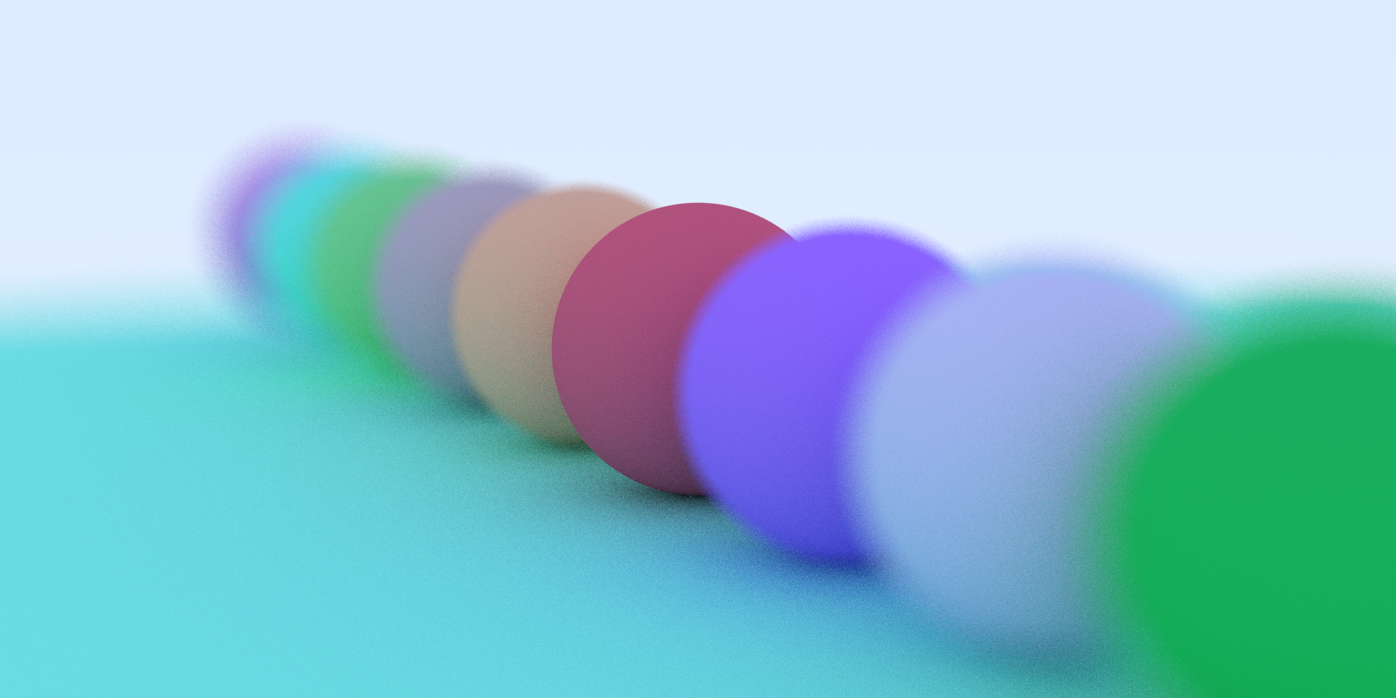
In optics, an aperture is a hole or an opening through which light travels. More specifically, the aperture and focal length of an optical system determine the cone angle of a bundle of rays that come to a focus in the image plane.

From the beginning, all scene rays have originated from look_from. To simulate a variable aperature, we’ll generate rays randomly originating from inside a disk centered at look_from. The larger we make this disc, the stronger the blur will be. With a disk radius of zero, the rays all originate from look_from, eliminating blur. One such method for generating a point inside a unit disk is as follows:

vec3.h:

vec3 random_unit_disk_coordinate() {
    while (true) {
        auto p = vec3(random_double(-1,1), random_double(-1,1), 0);
        if (p.length_squared() >= 1) continue;
        return p;
    }
}

Up until now, the focus distance was -1 on the z (or w) axes. We’ll now make it focus_distance and define our image plane accordingly:

lower_left_corner = origin - half_width*focus_distance*u - half_height*focus_distance*v - focus_distance*w;
horizontal = 2 * half_width*focus_distance*u;
vertical = 2 * half_height*focus_distance*v;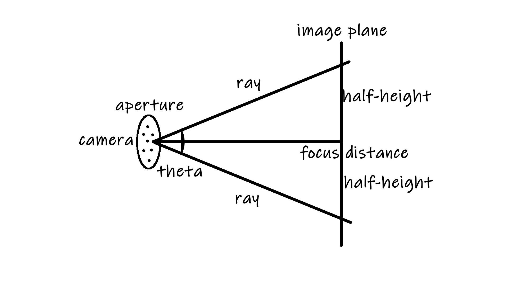

With that, we have a complete camera class:

camera.h

class camera {
    public:
        camera(vec3 look_from, vec3 look_at, vec3 vUp, double vFov, double aspect_ratio, double aperture, double focus_distance) {
            
            lens_radius = aperture / 2;
            
            double theta = vFov*pi/180;
            double half_height = tan(theta/2);
            double half_width = aspect_ratio * half_height;
            origin = look_from;
            
            w = unit_vector(look_from - look_at);
            u = unit_vector(cross(vUp, w));
            v = cross(w, u);

            lowerLeftCorner = origin
                              - half_width * focus_distance * u
                              - half_height * focus_distance * v
                              - focus_distance * w;
            horizontal = 2*half_width*focus_distance*u;
            vertical = 2*half_height*focus_distance*v;
        }

        ray get_ray(double s, double t) {
            vec3 rd = lens_radius*random_unit_disk_coordinate();
            vec3 offset = u * rd.x() + v * rd.y();

            return ray(origin + offset,
                       lowerLeftCorner + s*horizontal + t*vertical - origin - offset);
        }

        vec3 origin;
        vec3 lowerLeftCorner;
        vec3 horizontal;
        vec3 vertical;
        vec3 u, v, w;
        double lens_radius;
};

---

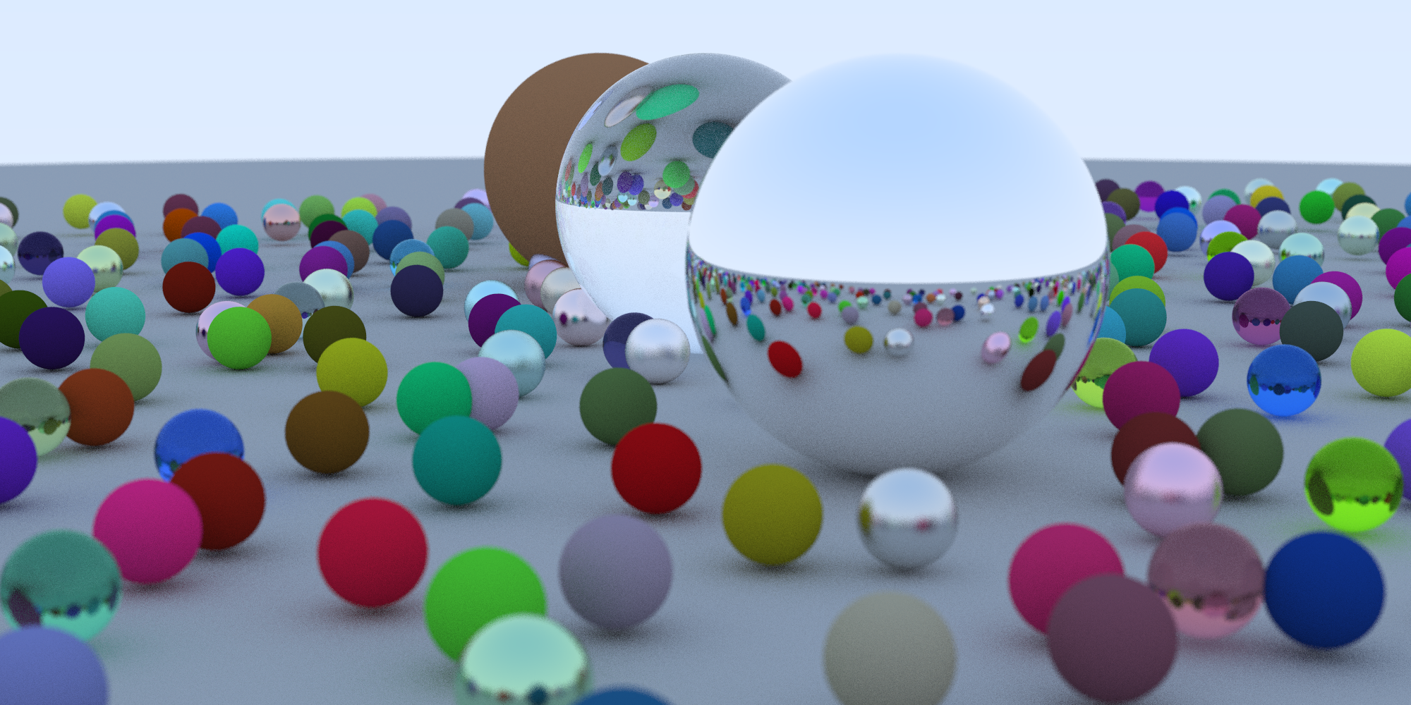
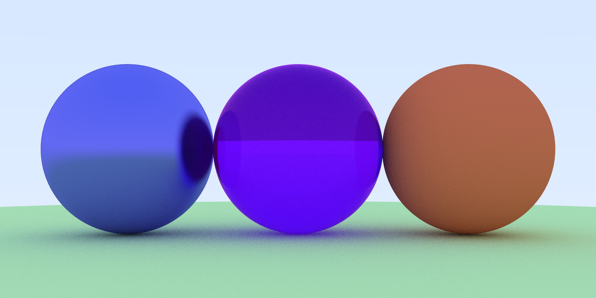
Final Scene

Lastly, we’ll create a random scene of spheres. Feel free to customize. And be aware - this may take some time to render!

main.cpp

...
hittable *random_scene() {
    int n = 500;
    hittable **list = new hittable*[n+1];
    list[0] =  new sphere(vec3(0,-1000,0), 1000, new lambertian(vec3(0.5, 0.5, 0.5))); // "Ground"
    int i = 1;
    for (int a = -11; a < 11; a++) {
        for (int b = -11; b < 11; b++) {
            double randomMaterial = random_double(0,1);
            vec3 center(a+0.9*random_double(0,1),0.2,b+0.9*random_double(0,1));
            if ((center-vec3(4,0.2,0)).length() > 0.9) {
                if (randomMaterial < 0.68) {  // diffuse
                    list[i++] = new sphere(center, 0.2,
                        new lambertian(vec3(random_double(0,1)*random_double(0,1),
                                            random_double(0,1)*random_double(0,1),
                                            random_double(0,1)*random_double(0,1))
                        )
                    );
                }
                else if (randomMaterial < 0.87) { // metal
                    list[i++] = new sphere(center, 0.2,
                            new metal(vec3(0.5*(1 + random_double(0,1)),
                                           0.5*(1 + random_double(0,1)),
                                           0.5*(1 + random_double(0,1))),
                                      0.5*random_double(0,1)));
                }
                else {  // glass
                    list[i++] = new sphere(center, 0.2, new dielectric(vec3(random_double(0,1),random_double(0,1),random_double(0,1)), 1.5));
                }
            }
        }
    }

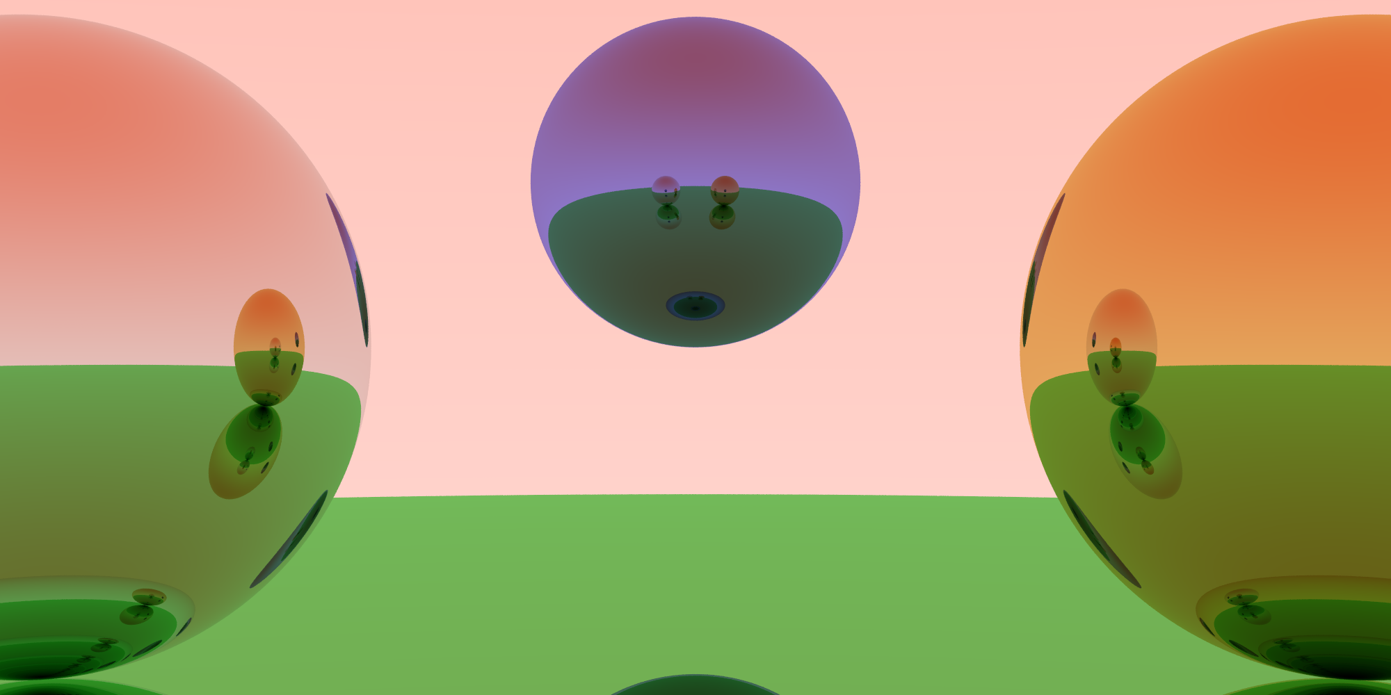
    list[i++] = new sphere(vec3(0, 1, 0), 1.0, new dielectric(vec3(1.0,1.0,1.0), 1.5));
    list[i++] = new sphere(vec3(-4, 1, 0), 1.0, new lambertian(vec3(0.4, 0.2, 0.1)));
    list[i++] = new sphere(vec3(4, 1, 0), 1.0, new metal(vec3(1.0, 1.0, 1.0), 0.0));

    return new hittable_list(list,i);
}

int main() {

...

double aperture = 0.2; // bigger = blurrier

    hittable *world = random_scene();

	camera cam(lookFrom, lookAt, vec3(0,1,0), 20,double(nx)/double(ny), aperture, distToFocus);
...
}
...

---

#graphics #ray-tracing-in-one-weekend #c++